Causal graph geodesics to continuous geodesics
Gene Chen
University of Maryland, College Park
Gene Chen
University of Maryland, College Park
What continuous properties we would see in a sample space of hypergraphs or causal networks? To approximate continuity, one could increase a graph’s size or, as this project’s approach, by taking an average over a multiple sprinkling. Given a causal graph constructed by a sprinkling procedure into an existing manifold, one can construct geodesics in the causal graph that approximate the geodesics in the associated space to an arbitrary degree of precision. This project investigates under what conditions we get stable convergence, instabilities, and how that affects the emergence of continuous geometry.
Purpose
Purpose
The Wolfram Model is a candidate for the fundamental theory of physics. It proposes hypergraphs as constituents of space while causal evolution of hypergraphs, or causal graphs, as spacetime. By discretizing spacetime, this model hopes to bridge general relativity and quantum mechanic. If hypergraphs and causal graphs are the forms of space and spacetime, they should recover our physical world in the continuous limit; in particular, this project focuses on how geodesics in causal graphs converge to the continuous geodesics. How the size of the graph and the number of graphs averaged affect the speed of convergence? How fast does geodesics within the light-cone converge compared to geodesics on the light-cone? Is it possible to determine the dimension of the manifold using light cones composed from individual geodesics? What are the obstructions and instability of convergence? These are questions this project aims to answer eventually (upon future updates).
Causal Graphs and discrete geodesics
Causal Graphs and discrete geodesics
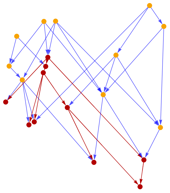
Causal graphs are made by sprinkling points on a vertex through the Poisson point process. For so far, all analysis is on 1+1 Dimension flat spacetime. The vertical axis represents time-like surfaces (time evolves downwards), while the horizontal represents space-like surfaces in the causal graph below. This embedded graph represents an arbitrary observer’s choice of coordinates where information of physical significance is encoded in the combinatorial structure of the graph, invariant under arbitrary embedding. The graph’s red portion shows a light-cone where all the vertices are causally connected to the uppermost red vertex, and nothing travels faster than 45°.
|
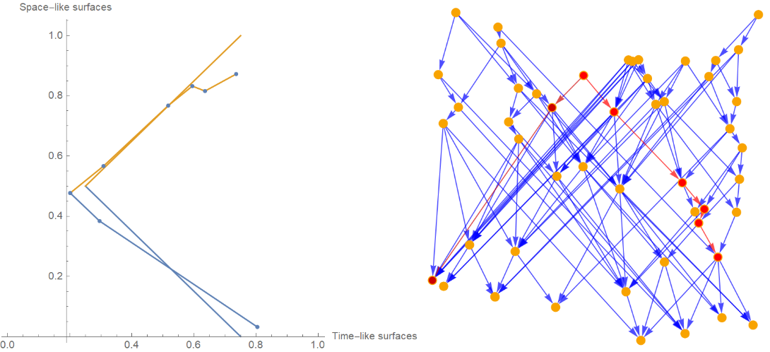
Geodesics in the hypergraph are defined by the vertices closest to the continuous geodesic endpoints in the embedded manifold. There would be cases where the endpoint is within the continuous light cone, but it remains causally disconnected to the starting point in the causal graph and doesn’t exist a geodesic between them. Such occurrences are beyond the intended scope of this project and ignored. The Left plot is a comparison between continuous and discrete light-like geodesics, forming a light-cone. By reflecting the left plot over x=0.5 and y=x, one can recover the geodesics highlighted in the causal graph on the right.
Averaging over discrete geodesics
Averaging over discrete geodesics
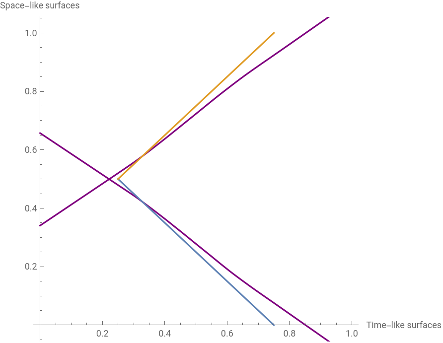
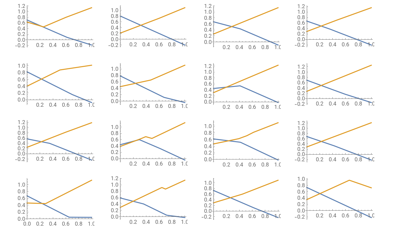
The plot below is derived by averaging over 200 discrete geodesics, with 70 sprinkled points each. The first 16 plots from the averaging are shown on the right. Since the continuous geodesic is light-like, the approximation could only underestimate the steepness of the geodesic. Apart from underestimating light-like geodesics, there isn’t any interesting obstruction to convergence observed so far. We anticipate instability towards convergence as we move on to a higher dimension manifold with curvature, which is yet to be investigated at this point.
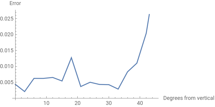
To quantify how good the approximation is, we define error = , integrated over the time-like surfaces of the continuous geodesic [0.25, 0.75]. The plot below compares the error of approximation for various geodesics from 0° (a vertical line in the causal graph) to 45° (light-like geodesic). Each point is averaging over 200 samples with 40 points each. We can see roughly that the geodesics near light-like are harder to approximate as expected.
∫
2
(continuousgeodesic-descretegeodesic)
size of the graph, number of graphs and the speed of convergence
size of the graph, number of graphs and the speed of convergence
Next, we go off tangent a bit to briefly investigate how the graph’s size and the number of graphs averaged affects convergence speed. Increasing the number of points is slightly more effective than increasing the sample size in the parameter range we choose.


Future directions
Future directions
Keywords
Keywords
◼
Causal Graph
◼
Discrete Math
Acknowledgment
Acknowledgment
Mentor: Nikolay Murzin
This project is impossible to do without the guidance from Nikolay Murzin and Jonathan Gorard. They helped me devised this interesting topic and taught me the basic physical intuition to make sense of it. I’m also thankful to Ruhi Shah who helped me with coding in mathematica.
References
References
◼
[1] Wolfram Physics Project: Technical Documentation. https://www.wolframphysics.org/technical-introduction/