Abstract: Chaos theory has introduced concepts like strange attractors, the Poincaré map, bifurcation dynamics, and the Mandelbrot set, shedding light on the relationship between determinism and unpredictability in complex systems. In the field of quantum mechanics, Bohm’s causal interpretation introduced a perspective on particle trajectories that provides a framework for the study of deterministic chaos at the quantum scale. Bohm’s theory combines the precision of causal quantum description with the intuitive insight arising from the formalism of trajectory description from classical mechanics, providing a powerful theoretical tool for understanding the physical mechanisms underlying microscopic phenomena. This article highlights the isotropic and anisotropic quantum harmonic oscillator as central models for exploring chaotic behavior at the quantum level, which means exponential divergence of neighbouring trajectories. Many methods of chaos theory can be applied to the investigation of Bohm’s trajectories. This article explores fundamental aspects of chaotic dynamics, quantified through the Lyapunov exponent, a key measure of sensitivity to initial conditions. A central focus is on Poincaré sections, which provide insight into the structure of trajectory evolution, and attractors, often exhibiting fractal properties. Chaos arises in regions where the wavefunction vanishes, defining nodal points that, along with saddle points (X-points), govern the system’s transition to unpredictability. Nodal points can be either stationary or moving, influencing the surrounding flow. Additionally, the fractal geometry of basin boundaries emerges when multiple nodal points undergo slight displacements, forming intricate regions of attraction where trajectories remain confined by the nodal structure and the underlying potential.
Together, these methods serve as essential tools for dissecting the complexities of quantum systems, shedding light on the interplay between determinism and unpredictability in their dynamics, and revealing deeper insights into the mechanisms that govern quantum chaos.
Together, these methods serve as essential tools for dissecting the complexities of quantum systems, shedding light on the interplay between determinism and unpredictability in their dynamics, and revealing deeper insights into the mechanisms that govern quantum chaos.
Full list of posts: https://community.wolfram.com/web/kvbloh/
Note: see the detailed introduction to the de Broglie Bohm theory with Mathematica here:
https://community.wolfram.com/groups/-/m/t/3000266
Note: see the detailed introduction to the de Broglie Bohm theory with Mathematica here:
https://community.wolfram.com/groups/-/m/t/3000266
1. Introduction
1. Introduction
Sometimes it is necessary to end a Wolfram Language kernel session or to clear all values, definitions, attributes, defaults, options and messages for the symbols.
In[]:=
Quit[]
In[]:=
ClearAll["Global`*"]
Use the following command, if you need to save/export graphs created by Mathematica into the current notebook directory:
In[]:=
SetDirectory[NotebookDirectory[]]
Out[]=
I:\Mathematica Notebooks
Cells that contain ‘dynamic content’ often lead to a system message. As a result, it is sometimes necessary to switch off dynamic evaluation for certain calculations.
PaletteNotebook@Column[{Button["Dynamic off",SetOptions[NotebookSelection[],DynamicUpdating->False]],Button["Dynamic on",SetOptions[NotebookSelection[],DynamicUpdating->True]]}]
In[]:=
SetOptions[$FrontEnd,"DynamicEvaluationTimeout"->30]
Feel free to use, reproduce, and modify this code in its entirety or in part of it. A further note: Some descriptions might be formulated too simply and could possibly require a more detailed explanation. I applied parallelization of the computational steps only in areas where a significant increase in processing speed could be achieved.
WARNING: These notes are incomplete and may contain errors in the implementation of the code and in the implementation of the equations. The essay has been written to the best of my knowledge and with great care. Every equation has been checked. It cannot be ruled out that errors may still exist. Some of the formulations are not introduced with mathematical precision and may contain linguistic inaccuracies. For simplicity, the SI units are not used at all. The author hopes, that readability is not significantly affected by this. The essay has not undergone a detailed peer review. Attention was paid to the clarity and comprehensibility of the equations. Therefore, many equations were not combined into a single expression. This sometimes results in less than optimal computational efficiency. They rather serve didactic purposes and aim to contribute to an understanding of handling mathematics with Mathematica. Similarly, I have not indicated quotes from my own works. To the best of my knowledge, I have listed all individuals from whom I have adopted parts of the programs. If I have overlooked people who have contributed to Bohm’s theory with regard to chaos theory or to the algorithms used, this is solely my responsibility. The literature list does not claim to be exhaustive with regard to all persons involved in the research of chaotic systems with Bohmian trajectories.
CAUTION! Enter parameters as rational numbers if possible, so that numerics are as accurate as possible.
2. Introduction to Chaos Theory
2. Introduction to Chaos Theory
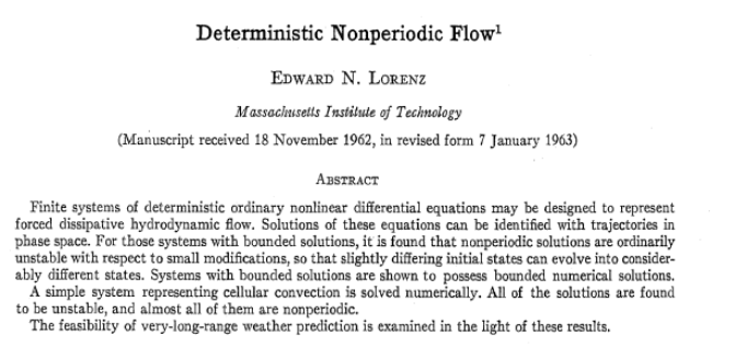
Chaos theory, significantly advanced by Edward Lorenz’s seminal work on ‘Deterministic Nonperiodic Flow’ and further developed through Benoît Mandelbrot’s studies of fractals and Mitchell Feigenbaum’s exploration of bifurcations, has revolutionized our understanding of complex systems. Lorenz’s 1963 work, while not the first to study chaotic behavior, remains the foundational contribution that consolidated chaos theory as a distinct field of study, inspiring extensive interdisciplinary research into the dynamics of unpredictability and determinism.
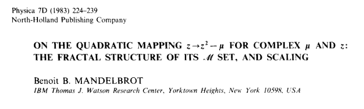
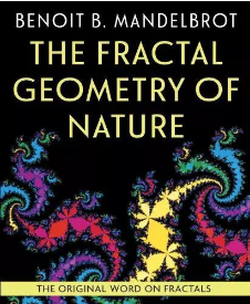
Benoît Mandelbrot played a pivotal role in this transformation by introducing fractals as mathematical tools capable of modeling natural irregularities such as coastlines, clouds, and mountain ranges. His seminal book, ‘The Fractal Geometry of Nature,’ demonstrated that fractals, characterized by self-similarity and fractional dimensions, were not merely abstract curiosities but crucial to understanding the inherent complexity of chaotic systems. Mandelbrot’s work bridged the gap between mathematics and the natural sciences, offering a framework to visualize and analyze phenomena that simultaneously exhibit order and randomness. The Mandelbrot Set, along with other core fractal concepts, became a cornerstone of chaos research, inspiring scientists to explore deeper connections between fractals, nonlinear dynamics, and chaotic behavior, thereby expanding the horizons of complexity science.
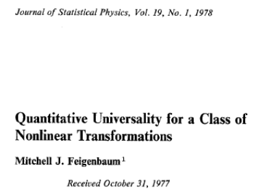
Mitchell Feigenbaum made another major contribution by uncovering the universal scaling laws that govern the bifurcation process in chaotic systems. His discovery of the Feigenbaum constants revealed that the transition to chaos follows a predictable, scaling pattern, offering insight into the underlying order behind chaotic behavior. Feigenbaum’s work on bifurcations and period-doubling cascades provided a crucial link between mathematical theory and physical systems, showing that chaos can emerge from simple, deterministic processes.
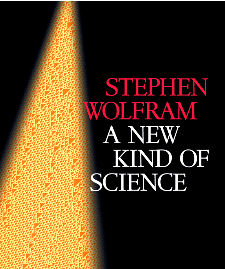
Stephen Wolfram’s work, particularly in ‘A New Kind of Science’, highlights how simple computational rules, like those in cellular automata, can generate complex and chaotic behavior. He demonstrated that such systems can model phenomena seen in nature, bridging computation and chaos theory. Wolfram’s ideas offer a new perspective on understanding complexity and unpredictability in natural systems.
These foundational works introduced key ideas such as strange attractors, bifurcation dynamics, and fractal structures that capture the unpredictable yet deterministic nature of chaotic systems. In quantum mechanics, Bohm’s causal interpretation provided a more intuitive perspective through the use of particle trajectories, laying the foundation for the study of deterministic chaos at the quantum scale. Central to this research are phenomena like the exponential divergence of neighboring trajectories, Poincaré sections and the Lyapunov exponent, which serve as quantitative measures of chaotic behavior.
-----------
----------
----------
Personal Remark by the Author: Mandelbrot’s book ‘The Fractal Geometry of Nature’ also awake my own fascination with the interplay between determinism and unpredictability in chaotic systems, including their exploration in causal quantum mechanics from the perspective of Bohmian trajectories. During the 1980s, Bremen was a leading center for chaos research. During my physics studies at the University of Bremen, I had the privilege of attending lectures and talks by prominent persons such as Michael Feigenbaum, Heinz-Otto Peitgen, and Peter H. Richter.
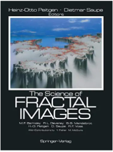
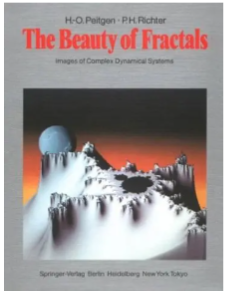
The University of Bremen holds a significant place in the history of chaos research, particularly through the pioneering work of mathematicians and physicists like Heinz-Otto Peitgen, Dietmar Saupe and Peter H. Richter. Their influential books, including ‘The Beauty of Fractals ‘ and ‘The Science of Fractals Images,’ played a major role in popularizing chaos theory and fractal geometry worldwide. These works not only provided deep insights into the mathematical underpinnings of chaos but also showcased its visual and structural beauty, making the field accessible to both scientists and the general public. The University of Bremen became a hub for interdisciplinary collaboration, fostering advancements in the visualization of complex systems and the application of chaos theory to diverse fields such as physics, biology,and economics.
3.Introduction Quantum Systems with Chaotic Bohmian Trajectories
3.Introduction Quantum Systems with Chaotic Bohmian Trajectories
Until the 1990s, there were no models that showed exponential divergence or sensitive dependence on initial conditions in the context of Bohmian trajectories, although David Bohm himself had suggested early on that such phenomena might be possible in his interpretation of quantum mechanics [20, Section 8.5 and Section 9.2]. Bohm speculated that the complex dynamics of the wavefunction, particularly in systems with multiple degrees of freedom, could lead to a sensitive dependence of the trajectories on their initial conditions, similar to classical chaos.
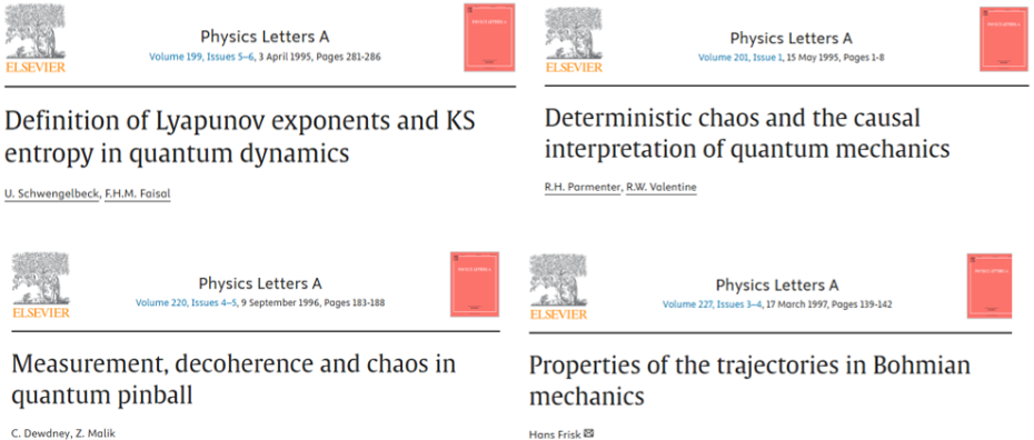
Early investigations in Bohmian mechanics were often limited to simple systems, such as the linear superposition of Gaussian waves or the tunnelling of a Gaussian wave function through a rectangular potential [18a, 18b], partly due to computer limitations. No signs of chaos or exponential divergence were observed in these models. In the 1990s, the search for chaotic Bohmian trajectories in quantum mechanics was of great significance because it promised deeper insights into the relationship between classical and quantum dynamical behavior. In [1] it was shown that if one considers the particles of a quantum system as ‘real’, i.e. if their positions are part of the state description, one obtains in principle a formulation in which the ‘quantum chaos’ also emerges from the dynamical law. The concept of deterministic chaos, central to classical nonlinear systems, raised the question of whether similar phenomena could occur in quantum mechanics, particularly within Bohmian mechanics. The possibility of finding chaotic Bohmian trajectories was crucial for testing the hypothesis that the apparent randomness of quantum mechanics might be rooted in deterministic but chaotic processes. Such a discovery could have bridged the gap between classical chaos theory and quantum mechanics, shedding light on the structure of configuration or phase space [25, 29] in quantum systems and enhancing our understanding of their dynamics. Additionally, the investigation of chaos in Bohmian trajectories provided an opportunity to critically examine Bohmian mechanics, explore its limitations, and compare its predictions with those of standard quantum mechanics. Chaotic behavior in Bohmian trajectories could also clarify the stability of trajectories and their role in quantum processes, particularly in the context of quantum chaos and the explanation of macroscopic quantum phenomena. Historically, the anisotropic harmonic oscillator[3a, 3b, 9], the infinite square well [5,6,7], circular billiard potential [8] and the isotropic harmonic oscillator[12, 13, 16] form the basis of chaotic Bohmian trajectories. These models provide a foundation for chaotic systems in the Bohmian approach. In [2], U. Schwengelbeck and F. H. M. Faisal gave a definition of quantum Lyapunov exponents and the associated KS entropy for a quantum delta-kicked rotator, which allows a rigorous characterisation of regular or irregular quantum dynamics using the same terms as in classical dynamics, where the quantum kicked rotator undergoes periodic “kicks” at discrete time intervals.
In the field of Bohmian mechanics for continuous and smooth wavefunctions, the research of chaotic Bohmian trajectories began with R. H. Parmenter and R. W. Valentine, who laid the foundation for the understanding of deterministic chaos in this framework in their paper ‘Deterministic Chaos and the Causal Interpretation of Quantum Mechanics,’ [3a, 3b]. They highlighted the critical role of eigenstate superposition and incommensurate eigenenergies in the emergence of quantum chaos. In a later paper [12], chaotic trajectories were found for a coupled isotropic harmonic oscillator. The frequencies are commensurable, but the amplitudes of the superimposed eigenfunctions have a complex relationship. Subsequently, C. Dewdney and Z. Malik identified a chaotic system in their work ‘Measurement, Decoherence, and Chaos in Quantum Pinball,’ [4] further advancing the study of chaotic behavior in quantum systems. Hans Frisk later built upon the ideas of Parmenter and Valentine in his article ‘Properties of the Trajectories in Bohmian Mechanics,’ [5] providing insights into the dynamics of Bohmian trajectories influenced by a constant phase shift. Later, an article by Goldstein showed that for systems limited to one dimension there is no exponential divergence and thus no chaotic behaviour in Bohmian trajectories[17], which is due, among other things, to the restriction of the well-known Bohmian non-crossing rule.
A significant advancement came with the works of D. A. Wisniacki and F. E. R. Pujals ‘,Motion of vortices implies chaos in Bohmian mechanics‘ [12], P. Falsaperla, G. Fonte, ‘On the motion of a single particle near a nodal line in the de Broglie–Bohm interpretation of quantum mechanics’ [11] and Efthymiopoulos, Kalapotharakos, and Contopoulos ’,Nodal points and the transition from ordered to chaotic Bohmian trajectories,’ [14] who identified nodal points (or nodal lines, called nodes)—regions where the wavefunction amplitude vanishes—and their associated X-points as critical structures characterising the transition from ordered to chaotic trajectories (Hopf bifurcation [14, 31]). Their research provided deeper insights into the mechanisms underlying quantum chaos and the intricate interplay between classical and quantum dynamics.
The present paper focuses on the two-dimensional, time-dependent of the ‘hydrodynamical’ probability flows, in short wave density flow or wave density, and streamlines of two independent harmonic oscillators, which are coupled by the total wavefunction, where the wavefunctions containing nodal points and, subsequently, multiple nodal points. The trajectories are determined and analyzed using methods from chaos theory to uncover the dynamic structures that govern their evolution.
Personal Note:
Without knowing Hans Frisk’s work at the time, I was working at the University of Portsmouth, England, in Chris Dewdney’s group on the same problem of superposition of eigenstates for a particle in a potential well with infinitely high walls in David Bohm’s trajectory description. Unfortunately for me and fortunately for Hans Frisk, Frisk published his results sooner (January 1997), so my results were only included in my PhD thesis (1998, University of Portsmouth, England, unpublished). But of course I was also proud that I had found a system in which the particle trajectories showed exponential divergence.
Without knowing Hans Frisk’s work at the time, I was working at the University of Portsmouth, England, in Chris Dewdney’s group on the same problem of superposition of eigenstates for a particle in a potential well with infinitely high walls in David Bohm’s trajectory description. Unfortunately for me and fortunately for Hans Frisk, Frisk published his results sooner (January 1997), so my results were only included in my PhD thesis (1998, University of Portsmouth, England, unpublished). But of course I was also proud that I had found a system in which the particle trajectories showed exponential divergence.
4. The Model: The Isotropic and the Anisotropic Harmonic Oscillator
4. The Model: The Isotropic and the Anisotropic Harmonic Oscillator
The isotropic harmonic oscillator is a fundamental model in quantum mechanics, representing one of the simplest systems where a particle experiences a restoring force proportional to its displacement from equilibrium. Its defining feature is symmetry, with identical oscillation frequencies in all spatial directions, leading to uniform behavior irrespective of orientation. This symmetry not only makes the model analytically solvable but also highly applicable as a starting point for understanding more complex quantum systems. As a cornerstone of theoretical physics, the isotropic harmonic oscillator provides a framework for studying a wide variety of quantum phenomena, from atomic vibrations and molecular dynamics to quantum field theory. Its well-defined energy levels and eigenstates make it an ideal system for exploring fundamental principles, including wave-particle duality and quantum coherence. Furthermore, the model’s symmetry properties offer insights into the role of invariance and conservation laws in quantum mechanics, which are essential for interpreting real-world physical systems.
In[]:=
EntityClass["PhysicalSystem","Quantum"]EntityList[%]
In[]:=
Entity["PhysicalSystem","IsotropicHarmonicOscillator2DCartesianCoordinates"][EntityProperty["PhysicalSystem","TimeDependentSchroedingerEquationPositionRepresentation"]]Entity["PhysicalSystem","IsotropicHarmonicOscillator2DCartesianCoordinates"][EntityProperty["PhysicalSystem","BoundStateWaveFunctionMomentumRepresentation"]]Entity["PhysicalSystem","IsotropicHarmonicOscillator2DCartesianCoordinates"][EntityProperty["PhysicalSystem","DiscreteEnergyEigenvalue"]]Entity["PhysicalSystem","IsotropicHarmonicOscillator2DCartesianCoordinates"][EntityProperty["PhysicalSystem","BoundStateWaveFunctionPositionRepresentation"]]
Out[]=
[,,](+)[,,]+[,,]+[,,]
(0,0,1)
Ψ
x
y
t
1
2
m
2
x
2
y
2
ω
Ψ
x
y
t
(0,2,0)
Ψ
x
y
t
(2,0,0)
Ψ
x
y
t
m
Out[]=
n
x
n
y
(-)
2
p
x
2
p
y
m
ω
n
x
p
x
m
ω
n
y
p
y
m
ω
π
n
x
n
y
2
n
x
n
y
m
ω
Out[]=
(1++)
ω
n
x
n
y
Out[]=
m
2
x
2
y
ω
n
x
x
HermiteHm
ω
n
y
y
m
ω
m
ω
π
n
x
n
y
2
n
x
n
y
The anisotropic harmonic oscillator extends the principles of the isotropic case by introducing different oscillation frequencies along each spatial direction. This breaks the symmetry of the system, allowing it to model environments with inherent directional dependencies or external influences that vary with orientation. As a result, the anisotropic harmonic oscillator becomes an indispensable tool for studying systems with non-uniform properties, such as crystals, layered materials, or particles confined in asymmetric traps.
In[]:=
Entity["PhysicalSystem","AnisotropicHarmonicOscillator2DCartesianCoordinates"][EntityProperty["PhysicalSystem","TimeDependentSchroedingerEquationPositionRepresentation"]]Entity["PhysicalSystem","AnisotropicHarmonicOscillator2DCartesianCoordinates"][EntityProperty["PhysicalSystem","BoundStateWaveFunctionMomentumRepresentation"]]Entity["PhysicalSystem","AnisotropicHarmonicOscillator2DCartesianCoordinates"][EntityProperty["PhysicalSystem","DiscreteEnergyEigenvalue"]]Entity["PhysicalSystem","AnisotropicHarmonicOscillator2DCartesianCoordinates"][EntityProperty["PhysicalSystem","BoundStateWaveFunctionPositionRepresentation"]]
Both models serve as the basis for Bohmian mechanics (for an introduction with Mathematica, see here). Using the eigenstates of the oscillator, this work investigates the deterministic trajectories of particles that can exhibit exponential divergence through superposition. The simplicity and symmetry of the isotropic harmonic oscillator make it an indispensable tool and forms the basis for the application of further concepts from chaos research.
5. Introduction to Bohmian mechanics
5. Introduction to Bohmian mechanics
8. Lyapunov Exponent for Bohmian Trajectories in an Anisotropic Harmonic Potential
8. Lyapunov Exponent for Bohmian Trajectories in an Anisotropic Harmonic Potential
8.1 The Model
8.1 The Model
8.2 Calculations of the Trajectories and the Lyapunov Exponents
8.2 Calculations of the Trajectories and the Lyapunov Exponents
The negative largest Lyapunov exponent indicates no exponential convergence of nearby trajectories. Small differences in initial conditions decay exponentially with time, leading to the suppression of any initial perturbations. This is characteristic of strongly stable systems, often due to dissipative effects or attractive fixed points in phase space. This is clearly seen by the periodic trajectory in the graphic above.
10. The Role of Nodal Points and X-Points in the Transition to Chaos
10. The Role of Nodal Points and X-Points in the Transition to Chaos
10.1 The Interaction between a Trajectories and Nodal Points at Rest
10.1 The Interaction between a Trajectories and Nodal Points at Rest
10.2 The Model
10.2 The Model
A ‘Resource’ function with the name ‘StationaryPoints’ is used to determine the minima and the saddle points.
The trajectories result from the gradients of the phase function, which, although the wave density is stationary, result from the constant phase shift of the eigenfunctions. The idea for the parallel computing was taken from Vitaliy Kaurov.
In many cases, Hopf bifurcations[14] of the orbits can be observed at saddle points. Trajectories near these critical points are stably attracted in one direction and unstably repelled in another. These critical points represent regions where the local dynamics of the system undergo a transition, causing trajectories in their vicinity to diverge. Neighboring trajectories, initially close in configuration space, are influenced by the competing dynamics of multiple basins of attraction. As a result, these trajectories are pulled toward different attractors, leading to an exponential separation of their paths over time.
10.3 The Interaction between a Trajectories and a Moving Nodal Point
10.3 The Interaction between a Trajectories and a Moving Nodal Point
Moving nodal points in quantum wavefunctions can be readily generated through the superposition of multiple eigenfunctions with different eigenenergies [9-16]. In such cases, the resulting wavefunction becomes time-dependent, leading to a time-dependent wave density. Consequently, the nodal points also become dynamic, moving through configuration space. These moving nodal points are accompanied by X-points, which adjust their positions in response to the nodal dynamics.
10.4 The Model
10.4 The Model
IMPORTANT: Performance Warning
The calculations and the creation of the ‘video frames’ can be very time-consuming due to the CPU capacity. It is recommended that you use the results specified at the beginning of the chapter. Save the results that you have created up to this point.
The calculations and the creation of the ‘video frames’ can be very time-consuming due to the CPU capacity. It is recommended that you use the results specified at the beginning of the chapter. Save the results that you have created up to this point.
Note: Sometimes it is necessary to restart the procedure for determining the Lyapunov exponent.
The Lyapunov exponent clearly shows the exponential divergence for this movement and is an indication of chaotic behaviour.
11. Stationary and Dynamic Nodal Points: The Fractal Geometry of the Basin Boundaries
11. Stationary and Dynamic Nodal Points: The Fractal Geometry of the Basin Boundaries
The concept of fractal patterns at the boundaries of basins of attraction is inspired by the idea described in the literature [1] using a magnetic pendulum. In this model, the pendulum is influenced by multiple magnets arranged below its plane of motion. Depending on the initial conditions, the pendulum ultimately settles near one of the magnets, corresponding to a specific basin of attraction. The boundaries of these basins exhibit fractal patterns, reflecting the system’s sensitivity to small changes in initial conditions. In Bohmian mechanics, a similar principle is applied to generate fractal basins of attraction, but based on the superposition of eigenstates for a degenerate wavefunction for the isotropic harmonic oscillator.
The fractal geometry of the basin boundaries can be shown by superimposing eigenstates where moving nodal points shift only slightly. Stationary nodal points are characterised by their fixed positions in configuration space, while dynamical nodal points move on well-defined, often circular or elliptical-like orbits (see, for example video [7]). This interplay creates a delicate balance of attraction and repulsion. These bifurcations allow the trajectories to shift into another basin of attraction, creating complex patterns in configuration space.
The fractal geometry of the basin boundaries can be shown by superimposing eigenstates where moving nodal points shift only slightly. Stationary nodal points are characterised by their fixed positions in configuration space, while dynamical nodal points move on well-defined, often circular or elliptical-like orbits (see, for example video [7]). This interplay creates a delicate balance of attraction and repulsion. These bifurcations allow the trajectories to shift into another basin of attraction, creating complex patterns in configuration space.
11.2 Poincaré Section
11.2 Poincaré Section
In order to generate the fractal patterns as a function of the initial values, it is necessary to calculate a large number of trajectories. The option of parallel calculation can be used here. The calculation of the trajectories for approx. 22,800 starting points requires approx. 100 seconds of computing time, whereby the number of kernels and the processing speed strongly influence the computing time. A large amount of memory (RAM) is also required.
IMPORTANT: Performance Warning
The calculations can be very time-consuming due to the CPU capacity. If AccuracyGoal, PrecisionGoal, and MaxSteps are increased, the results become even more precise, but at the expense of computing time.
The calculations can be very time-consuming due to the CPU capacity. If AccuracyGoal, PrecisionGoal, and MaxSteps are increased, the results become even more precise, but at the expense of computing time.
11.3 Color Mapping
11.3 Color Mapping
The five basins of attraction act as regions where the trajectories ultimately converge after sufficient time, leaving only five distinct “endpoint zones” corresponding to the system’s attractors. Each of these zones is represented by a unique color, and through a “color mapping” technique, the initial points in the phase space are colored according to their corresponding endpoint zones. The intricate, chaotic motion of the trajectories results in fractal structures at the boundaries of the basins, highlighting the system’s sensitive dependence on initial conditions.
If you want to check each assignment of the colours to the respective trajectories, start the animation below.
References
References
A heartfelt thank you to the Wolfram Team for their invaluable support in developing my programs with Mathematica. I am especially grateful to Vitaliy Kaurov and Ahmed Elbanna for their expert guidance and patience throughout the entire project.
A selection of animations can be seen in some of the author’s videos (Other Internet Sources: [1-8]).
A selection of animations can be seen in some of the author’s videos (Other Internet Sources: [1-8]).
Wolfram Demonstrations by Klaus von Bloh
Wolfram Demonstrations by Klaus von Bloh
Wolfram Community posts by Klaus von Bloh
Wolfram Community posts by Klaus von Bloh
Articles
Articles
[1] D. Dürr, S. Goldstein and N. Zanghi, “Quantum Chaos, Classical Randomness, and Bohmian Mechanics,” Journal of Statistical Physics, 68, 1992 p. 259-270. doi:10.1007/BF01048845.
[2] U. Schwengelbeck, F. H. M. Faisal, “Definition of Lyapunov exponents and KS entropy in quantum dynamics," Physics Letters A, 199(5–6), 1995 p. 281-286. doi:10.1016/0375-9601(95)00122-J.
[3a] R. H. Parmenter and R. W. Valentine, “Deterministic Chaos and the Causal Interpretation of Quantum Mechanics,” Physics Letters A, 201(1), 1995 pp. 1–8. doi:10.1016/0375-9601(95)00190-E.
[3b] R. H. Parmenter and R. W. Valentine, "Erratum: Deterministic Chaos and the Causal Interpretation of Quantum Mechanics," Physics Letters A, 213(5–6), 1996 p. 319. doi:10.1016/0375-9601(96)00096-5.
[4] C. Dewdney and Z. Malik, “Measurement, decoherence and chaos in quantum pinball,” Physics Letters A, 220(4-5), 1996 pp. 183–188. doi:10.1016/0375-9601(96)00533-6.
[5] H. Frisk,”Properties of the trajectories in Bohmian mechanics,” Physics Letters A, 227(3-4), 1997 p. 139-142. doi:10.1016/S0375-9601(97)00044-3.
[6] S. Konkel, A.J. Makowski, “Regular and chaotic causal trajectories for the Bohm potential in a restricted space,” Physics Letters A, 238(2-3), 1998 pp. 95–100. doi:10.1016/S0375-9601(97)00881-5.
[7] Hua Wu, D. W. L. Sprung, “Quantum chaos in terms of Bohm trajectories,” Physics Letters A, 261(3-4), 1999 pp. 150–157. doi:10.1016/0375-9601(96)00533-6.
[8] O. F. de Alcantara Bonfim, J. Florencio and F. C. Sá Barreto, "Chaotic Bohm’s Trajectories in a Quantum Circular Billiard," Physics Letters A, 277(3), 2000 pp. 129–134. doi:10.1016/S0375-9601(00)00705-2.
[9] A. J. Makowski and M. Frackowiak, "The Simplest Non-trivial Model of Chaotic Causal Dynamics," Acta Physica Polonica B 32, 2001 pp. 2831–2842. arXiv: 0111155v1 [quant-ph].
[11] P. Falsaperla, G. Fonte, “On the motion of a single particle near a nodal line in the de Broglie–Bohm interpretation of quantum mechanics,” Physics Letters A, 316(6), 2003 pp. 382–390. doi:10.1016/j.physleta.2003.08.010.
[12] D. A. Wisniacki and F. E. R. Pujals, “Motion of vortices implies chaos in Bohmian mechanics,” Europhysics Letters, 71 (2), 2005 pp. 159–166. doi:10.1209/epl/i2005-10085-3. arxiv:0502108[quant-ph].
[13] D . A . Wisniacki, E . R . Pujals, F . Borondo,”Vortex interaction, chaos and quantum probabilities,” Europhysics Letters, 73 (5), 2006. doi:10.1209/epl/i2005-10467-5. arXiv:nlin/0507015 [nlin.CD]
[14] C. Efthymiopoulos, C. Kalapotharakos and G. Contopoulos, "Nodal Points and the Transition from Ordered to Chaotic Bohmian Trajectories," Journal of Physics A: Mathematical and Theoretical, 40(43), 2007 12945. doi:10.1088/1751-8113/40/43/008. arXiv:0709.2038 [quant-ph].
[15] C. Efthymiopoulos, C. Kalapotharakos, and G. Contopoulos, "Origin of Chaos near Critical Points of the Quantum Flow," Physical Review E 79, 2009 pp. 036203-1–036203-18. doi:10.1103/PhysRevE.79.036203, arXiv: 0903.2655 [quant-ph].
[16] F. Borondo, A. Luque, J. Villanueva and D. A. Wisniacki, “A dynamical systems approach to Bohmian trajectories in a 2D harmonic oscillator," Journal of Physics A: Mathematical and Theoretical, 42(49), 2009 495103. doi: 10.1088/1751-8113/42/49/495103. arXiv:0907.0534 [quant-ph].
[17] S. Goldstein, “Absence of chaos in Bohmian dynamics,” Physical Review E 60, 1999. doi:10.1103/PhysRevE.60.7578. arXiv:quant-ph/9901005v1.
[18a] C. Dewdney and B. J. Hiley, “A Quantum Potential Description of One-Dimensional Time-Dependent Scattering from Square Barriers and Square Wells,” Foundations of Physics 12(1), 1982 pp. 27–48. doi: 10.1007/BF00726873.
[18b] C. Philippidis, C. Dewdney and B. J. Hiley, “Quantum Interference and the Quantum Potential,” Il Nuovo Cimento B Series 11, 52(1), 1979 pp. 15–28. doi:10.1007/BF02743566.
[19a] D. Bohm, “A suggested Interpretation of the Quantum Theory in Terms of Hidden Variables, I,” Physical Review 85 (2), 1952 pp. 166–179. doi:10.1103/PhysRev.85.166.
[19b] D. Bohm, “A suggested Interpretation of the Quantum Theory in Terms of Hidden Variables, II,” Physical Review 85 (2), 1952 pp. 180–193. doi:10.1103/PhysRev.85.18.
[20] D. Bohm and B. J. Hiley, The Undivided Universe, New York: Routledge, 1993. doi:10.4324/9780203980385.
[21] P . R . Holland, The Quantum Theory of Motion: An Account of the de Broglie–Bohm Causal Interpretation of Quantum Mechanics, New York : Cambridge University Press, 1993.
[22\b] S. Goldstein. “Bohmian Mechanics.” The Stanford Encyclopedia of Philosophy. (Jan 4, 2025) plato.stanford.edu/entries/qm-bohm.
[24] D.Bohm and J.P. Vigier, “Model of the Causal Interpretation of Quantum Theory in Terms of a Fluid with Irregular Fluctuations,” Physical Review 96(20), 1954 pp. 208–216. doi:10.1103/PhysRev.96.208.
[25] Wikipedia. “ Configuration space.” (Jan 4, 2025) https://en.wikipedia.org/wiki/Configuration_space_(physics).
[26] Wikipedia. “Aleksandr Lyapunov.” (Jan 4, 2025) https://en.wikipedia.org/wiki/Aleksandr_Lyapunov.
[27] Wikipedia. “ Ljapunow-Exponent.” (Jan 4, 2025) https://en.wikipedia.org/wiki/Lyapunov_exponent.
Chaos
Chaos
[1] H-O. Peitgen, H. Jürgens and D. Saupe, Chaos. Bausteine der Ordnung, Berlin Heidelberg: Springer-Verlag, 1994.
Other Demonstrations and internet sources
Other Demonstrations and internet sources
YouTube Internet Sources:
[1] K. von Bloh. Influence of Nodal Points in Bohmian Mechanics. [Video]. (Jan 28, 2025) https://www.youtube.com/watch?v=2fSKL6XpuGg&t=10s.
[2] K. von Bloh. Bohm Trajectories for a Particle in a Two Dimensional Circular Billiard. [Video]. (Jan 28, 2025) https://www.youtube.com/watch?v=7UBUxAcSFdc.
[3] K. von Bloh. Periodic Quantum Trajectories from Coherent States of the Poeschl Teller Potential. [Video]. (Jan 28, 2025) https://www.youtube.com/watch?v=qKw7NChAFgg.
[4] K. von Bloh. Weak Ergodic Quantum Trajectories from Coherent States of the Pöschl Teller Potential. [Video]. (Jan 28, 2025) https://www.youtube.com/watch?v=wVG7-NvHqJQ.
[5] K. von Bloh. Chaotic Bohmian Quantum Trajectories from Coherent States of the Poeschl-Teller Potential. [Video]. (Jan 28, 2025)https://www.youtube.com/watch?v=FsAtg5Ss0GU&t=59s.
[6] K. von Bloh. Quantum Motion in an Infinite Spherical Well. [Video]. (Jan 28, 2025) https://www.youtube.com/watch?v=X2GlCdjpTwo&t=43s.
[7] K. von Bloh. The Elliptical Orbit of a Nodal Point and the Influence on Causal Trajectories. [Video]. (Jan 28, 2025) https://www.youtube.com/watch?v=Il0xg4K-Y-g.
[8] K. von Bloh. Bohm Trajectories for a Particle in a Two-dimensional Calogero–Moser Potential. [Video]. (Jan 28, 2025) https://www.youtube.com/watch?v=M9TJmZMgLgQ.
CITE THIS NOTEBOOK
CITE THIS NOTEBOOK
Chaotic Dynamics in the Causal Interpretation of quantum mechanics
by Klaus von Bloh
Wolfram Community, STAFF PICKS, February 6, 2025
https://community.wolfram.com/groups/-/m/t/3382372
by Klaus von Bloh
Wolfram Community, STAFF PICKS, February 6, 2025
https://community.wolfram.com/groups/-/m/t/3382372