Wolfram Cloud Document

ABSTRACT (original article): To quantify the immune response against a rapidly evolving virus, groups routinely measure antibody inhibition against many virus variants. Over time, the variants being studied change, and there is a need for methods that infer missing interactions and distinguish between confident predictions and hallucinations. Here, we develop a matrix completion framework that uses patterns in antibody-virus inhibition to infer the value and confidence of unmeasured interactions. This same approach can combine general datasets—from drug-cell interactions to user movie preferences—that have partially overlapping features. CITATION (original article): Einav, Tal et al. (2023), Using interpretable machine learning to extend heterogeneous antibody-virus datasets, Cell Reports Methods, Volume 3, Issue 8, 100540. https://doi.org/10.1016/j.crmeth.2023.100540
GitHub: https://github.com/TalEinav/CrossStudyCompletion

Highlights

◼

Predict unmeasured antibody-virus interactions across multiple studies

◼

Empower direct comparisons between studies through expanded virus panels

◼

Determine which criteria (age, exposure history) lead to distinct responses

◼

Assess how accurately animal data predict the human antibody response

Summary

A central challenge in biology is to use existing measurements to predict the outcomes of future experiments. For the rapidly evolving influenza virus, variants examined in one study will often have little to no overlap with other studies, making it difficult to discern patterns or unify datasets. We develop a computational framework that predicts how an antibody or serum would inhibit any variant from any other study. We validate this method using hemagglutination inhibition data from seven studies and predict 2,000,000 new values ± uncertainties. Our analysis quantifies the transferability between vaccination and infection studies in humans and ferrets, shows that serum potency is negatively correlated with breadth, and provides a tool for pandemic preparedness. In essence, this approach enables a shift in perspective when analyzing data from “what you see is what you get” into “what anyone sees is what everyone gets.”

The following code reproduces the plots in the main text. Made on Mathematica version 13.2.0 for Windows. Sections can be opened by mouse click.

Raw data can be found in Matrix Completion section.

Figures

Accessing the Data

In this work, we analyze seven large influenza datasets measuring serum-virus inhibition. Values represent hemagglutination inhibition (HAI) titers, with larger values representing stronger antibody inhibition. We refer to these datasets in the code as follows:

◼

table="S1"

: Fonville Table S1, called

Dataset

Ferret

in our paper

◼

table="S3"

: Fonville Table S3, called

Dataset

Infect,1

in our paper

◼

table="S5"

: Fonville Table S5, called

Dataset

Vac,1

in our paper

◼

table="S6"

: Fonville Table S6, called

Dataset

Vac,2

in our paper

◼

table="S13"

: Fonville Table S13, called

Dataset

Vac,3

in our paper

◼

table="S14"

: Fonville Table S14, called

Dataset

Vac,4

in our paper

◼

table="Vinh"

: Vinh Dataset, called

Dataset

Infect,2

in our paper

Fonville 2014

For each dataset, the variables

viruses

and

sera

contain all the viruses and sera in that study. For example, here are the viruses and sera in Table S1

In[]:=

viruses["S1"]//Shortsera["S1"]//Short

Out[]//Short=

{NL/179/93,A/WELLINGTON/1/94,A/BRISBANE/22/94,68,VN020/EL443/2010,VN021/EL444/2010,VN053/2010}

Out[]//Short=

{Serum_A/WELLINGTON/25/93_TableS1,Serum_A/WELLINGTON/96/93_TableS1,32,Serum_A/HONGKONG/34/90_TableS1}

The sera are all labeled with their associated table for easy reference. Sera from Tables S5, S6, S13, and S14 [the vaccination studies] also have “_Pre” or “_Post” appended to their names to denote whether they were drawn pre- or post-vaccination. Below is one example from each Fonville study

In[]:=

First/@sera/@fonvilleTables//Column

Out[]=

Serum_A/WELLINGTON/25/93_TableS1

Subject1Year2007_TableS3

Subject258Age29_TableS5_Pre

Subject71Age18_TableS6_Pre

SubjectA028_TableS13_Pre

SubjectB007_TableS14_Pre

For convenience, the table index

All

can be used to get a list of the viruses or sera in all Fonville studies

In[]:=

viruses[All]//Shortsera[All]//Short

Out[]//Short=

{A/AUCKLAND/20/2003,A/AUCKLAND/5/96,A/BANGKOK/1/97,75,VN020/EL443/2010,VN021/EL444/2010,VN053/2010}

Out[]//Short=

{Serum_A/WELLINGTON/25/93_TableS1,Serum_A/WELLINGTON/96/93_TableS1,1144,SubjectB039_TableS14_Post}

Measurements are accessed via the

data

master function. As shown below, every virus-serum pair from the same table will either have a measurement or will be

Missing[]

. If a virus was not included in a table, then its interaction with a serum will not evaluate. Below are examples of each type of evaluation

In[]:=

data[{viruses["S1"][[1]],sera["S1"][[1]]}]data[{viruses["S1"][[-1]],sera["S1"][[1]]}]data[{viruses["S3"][[1]],sera["S1"][[1]]}]

Out[]=

640.

Out[]=

Missing[]

Out[]=

data[{BI/16190/68,Serum_A/WELLINGTON/25/93_TableS1}]

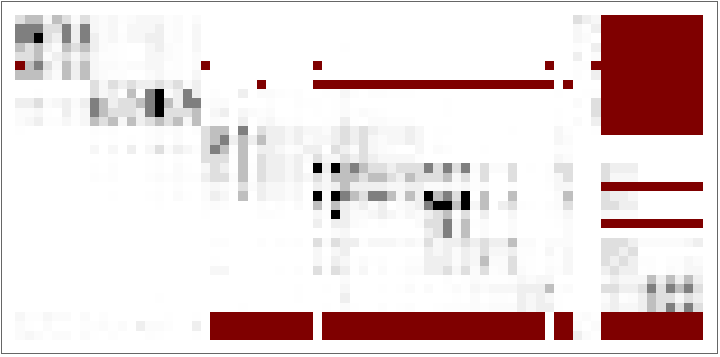
The code below displays all measurements from Table S1 as an ArrayPlot, with missing measurements shown in dark-red

In[]:=

(*Rawdata*)ArrayPlot@Table[data[{virus,serum}],{serum,sera["S1"]},{virus,viruses["S1"]}]

Out[]=

The following grid shows the number of sera and viruses in each Fonville Study

In[]:=

showGrid[Prepend[{#,Length@sera[#],Length@viruses[#]}&/@fonvilleTables,{"Study"," of Sera"," of Viruses"}]]

Out[]=

Study	 of Sera	 of Viruses
S1	35	74
S3	324	57
S5	212	70
S6	256	70
S13	160	20
S14	160	20

Vinh 2021

The Vinh dataset can be accessed just like the Fonville datasets using the

data

master function

In[]:=

data[{viruses["Vinh"][[1]],sera["Vinh"][[1]]}]

Out[]=

1810.

Below is the number of viruses and sera in the long-and-skinny Vinh dataset

◼

The full Vinh dataset contains 24,400 (10x more) sera than what is shown below. In this notebook, we only load every 10th Vinh serum to speed up initialization. The full Vinh serum can be loaded in the Initialization section

In[]:=

Echo[Length@viruses["Vinh"]," of Viruses in Vinh"];Echo[Length@sera["Vinh"]," of Sera in Vinh"];

 of Viruses in Vinh6

 of Sera in Vinh2440

An Anecdote showing the Power of Matrix Completion


Figure 3: Completion across Two Datasets

Our algorithm is built upon predicting virus behavior between pairs of studies, and we begin by considering three pairs from Fonville 2014.

◼

Panel A predicts between two human vaccination datasets [Fonville Table S13S14]

◼

Panel B predicts between human infection and vaccination data [Fonville Table S3S14]

◼

Panel C predicts between ferret infection and human vaccination data [Fonville Table S1S14]

Notes about the code:

◼

The first element mapped over,

{"S13"->"S14",10}

, states that we predict from Table S13S14 values for

viruses["S14"][[10]]="A/AUCKLAND/5/96"

◼

"OtherTables"->{tablePredictingFrom}

specifies that only Table S13 should be used to make these predictions. (The default behavior is to use all other tables)

◼

"PlotType"->"Swarm"

shows the output as a swarm plot, which is necessary for Fonville predictions because they take on discrete values (5, 10, 20...) that all collapse in a normal scatterplot

◼

In Figure S2, we systematically predict the values for all other viruses in Table S14 from these three tables

◼

To decrease file size, we use a trimmed forest with less accurate predictions [described in the Initialization section]

In[]:=

GridTranspose@MapIndexed{tablePredictingFrom,tableOfInterest}=List@@#[[1]];virusOfInterest=viruses[tableOfInterest][[#[[2]]]];plotCompletioncompletionPredictions[{virusOfInterest,tableOfInterest},"OtherTables"->{tablePredictingFrom}],"PlotType"->"Swarm",

&,(*Predictingfrom{TableXTableY,Viruswiththisindex}*){{"S13"->"S14",10},{"S3"->"S14",5},{"S1"->"S14",17}},Spacings->{2,2}

Out[]=

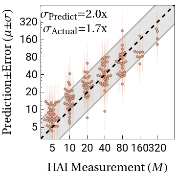
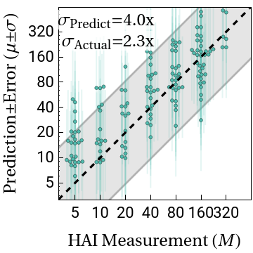
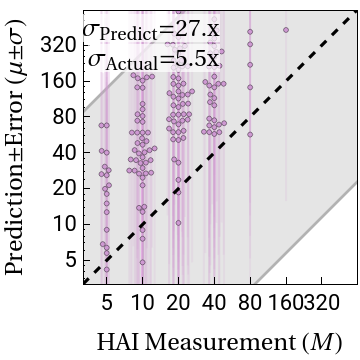
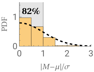
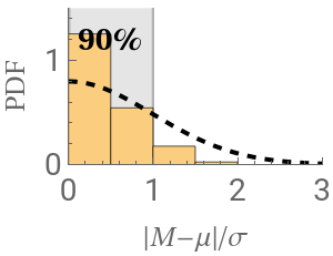
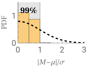
Figure 4: Leave-One-Out Analysis

We perform leave-one-out analysis, where one virus is entirely withheld from a dataset, and its values are predicted using the remaining datasets. In total, we predict 317 virus-dataset pairs, predicting 200,000 measurements.

Panel A: Schematics of the Data

Below are schematics of each dataset that we analyze. Note that the Vinh dataset is so long (25,000 sera) that we only show every 10th serum, and even so it is extremely long-and-skinny. Measurements are shown in grayscale while missing values are shown in dark-red.

Panel A: Prediction Scatter Plots

Panel B: Chord Diagram

We summarize the transferability between datasets using a chord diagram. For each arc connecting datasets X and Y, a larger width at the outer circle represents greater transferability. Notes on this code:

◼

Transferability is not symmetric between tables, and hence the two widths are generally different

◼

Tables are labeled according to their original source [see the translation here]

◼

Note that the Fonville Ferret Study is poorly predicted by all other tables, and hence it has no appreciable transferability

Figure 5: Leave-Multi-Out Analysis

In Figure 3, we showed that multiple viruses can be individually withheld and accurately predicted via matrix completion. Here, we demonstrate that a large set of 124 viruses can be simultaneously withheld and predicted.

Panel A: Schematics of the Data

The schematics below depicts the 124 viruses [shown in gold] that we simultaneously withheld from the various datasets.

Panel A: Prediction Scatter Plots

As in Figure 3A, we show scatter plots comparing the leave-multi-out predictions to the actual measurements.

◼

Note that in this leave-multi-out analysis, we simultaneously predict the 70,000 measurements from 124 viruses

◼

In contrast, during leave-one-out analysis we only withhold a single virus, predicting far fewer measurements (on the order of hundreds)

Panel B: Chord Diagram

As in Figure 3B, we summarize the transferability between datasets using a chord diagram. This diagram looks markedly different from the main text result because we used trimmed forests in this notebook.

Figure 6: Expanding Datasets

Here, we expand the Fonville and Vinh dataset as much as possible, predicting each of their sera against all 81 viruses that appears in these datasets. This expansion requires an additional random forest whose creation is described in the Initialization section.

Extending Vinh Data

The Vinh dataset reaps the greatest benefits from this expansion, since it contains many sera and few viruses. By predicting how the 25,000 Vinh sera inhibit 75 additional viruses, we predict 2,000,000 new measurements.

◼

Note that we only load every 10th Vinh serum to increase the speed of these predictions, which is why the y-axis shows values that are 10x smaller than what we have in the manuscript [this can be undone in the Initialization section]

Extending Fonville Panel

Figure 7: Applications of Matrix Completion

We present a few potential applications using the expanded antibody-virus measurements, although we hope that this wealth of data will serve as the springboard for many additional forms of analysis.

Panel A: High-Resolution Antibody Response

Three examples of the expanded antibody response

◼

Since we only load every 10th Vinh serum for speed, the Vinh landscape slightly differs although it shows the same trend. (If the full Vinh dataset were loaded, the 5th serum would show the response from the manuscript)

Panel B: Breadth vs Potency

Panel C: Pandemic Preparedness: New Variant Arises, Measured in 1 Dataset

H3N2 Perth 2009 is the most recent virus in the most recent dataset (Fonville S14). If this virus just emerged and was only measured in S14, could we predict its values in S13 to see whether those sera would also inhibit this new variant?

Figure S4: Explaining the Chord Diagrams

◼

Transferability is clipped to lie between 0 and 1, where 0 represents poor transferability and 1 represents two datasets with perfect transferability

Figure S7: Visualizing the Expanded Datasets

We show all of the values in the expanded Fonville and Vinh datasets that can be predicted with ≤4-fold error. The Vinh predictions may look artificially different from the main text figure because sera are clustered based on their similarity, and the orders of clusters may change.

Figure S9: UMAP of Expanded Datasets

Using the expanded datasets, we can apply a UMAP and overlay the (unused) information about each virus’s year of circulation to examine whether the viruses evolve in time towards distinct patterns

◼

Because we only use every 10th Vinh serum for speed, the Extended Vinh plot looks slightly different from what is shown in the manuscript

Initialization

Code for growing forests of decision trees is attached below

CITE THIS NOTEBOOK

Using interpretable machine learning to extend heterogeneous antibody-virus datasets
by Tal Einav & Rong Ma
Wolfram Community, STAFF PICKS, October 3, 2025
https://community.wolfram.com/groups/-/m/t/3555650

Figures

Accessing the Data

Fonville 2014

Vinh 2021

An Anecdote showing the Power of Matrix Completion

Figure 3: Completion across Two Datasets

Figure 4: Leave-One-Out Analysis

Panel A: Schematics of the Data

Panel A: Prediction Scatter Plots

Panel B: Chord Diagram

Figure 5: Leave-Multi-Out Analysis

Panel A: Schematics of the Data

Panel A: Prediction Scatter Plots

Panel B: Chord Diagram

Figure 6: Expanding Datasets

Extending Vinh Data

Extending Fonville Panel

Figure 7: Applications of Matrix Completion

Panel A: High-Resolution Antibody Response

Panel B: Breadth vs Potency

Panel C: Pandemic Preparedness: New Variant Arises, Measured in 1 Dataset

Figure S4: Explaining the Chord Diagrams

Figure S7: Visualizing the Expanded Datasets

Figure S9: UMAP of Expanded Datasets

CITE THIS NOTEBOOK

An Anecdote showing the Power of Matrix Completion
