Thermodynamic Cycle OptimizationAuthors: Gino J. A. de Andrade (Federal University of Amazon, gandrade@ufam.edu.br) Rubelmar Cruz Neto (Amazon State University, rcruzneto@uea.edu.br)
Data Source
Data Source
In[]:=
A=;fun[col_]:=Transpose@{A[[2;;,1]],A[[2;;,col]]};DataPxT=Transpose@{A[[2;;,1]],A[[2;;,2]]};DataTxP=Transpose@{A[[2;;,2]],A[[2;;,1]]};{DatavlxT,DatavvxT,DataulxT,DatauvxT,DatahlxT,DatahvxT,DataslxT,DatasvxT}=Table[Transpose@{A[[2;;,1]],A[[2;;,col]]},{col,3,10}];{press,Temp,vl,vv,ul,uv,hl,hv,sl,sv}=Interpolation[#,InterpolationOrder1]&/@{DataPxT,DataTxP,DatavlxT,DatavvxT,DataulxT,DatauvxT,DatahlxT,DatahvxT,DataslxT,DatasvxT};dataEnthalpySuperHeated=;dataEntropySuperHeated=;{enthalpySuperHeated,entropySuperHeated}=Interpolation[#,InterpolationOrder1]&/@{dataEnthalpySuperHeated,dataEntropySuperHeated};vaporQuality[t_,s_]:=(s-sl[t])/(sv[t]-sl[t])//N;
ThermodynamicaCycle
ThermodynamicaCycle
In this part we have the ThermodynamicCycle function. It is a function I coded during Wolfram Summer School 2020 that returns values of performance parameter and properties at each thermodyanamic state. User should input a few properties, then the function returns an object that contain parameters of the cycle. The code presented here is only realated to the Rankine Cycle.
In[]:=
Options[ThermodynamicCycle]={};ThermodynamicCycle[cycle:"RankineCycle",fluid:"Water",setting:{__Rule},opts:OptionsPattern[]]:=Module{p,T,T4,u,v,s,h,p1,p2,x2,eff,enthalpy,entropy,volume,temperature,pressure,wcycle,bwr,higherPressure,higherTemperature,lowerPressure,boilerTemperature,thermalEfficiency,workNet,workPerMass,HeatInput,HeatOutput},{higherPressure,higherTemperature,lowerPressure,boilerTemperature}=Replace[{"HigherPressure","HigherTemperature","LowerPressure","BoilerTemperature"},Append[setting,_Missing[]],{1}];T=Table[0,4];s=v=h=p=T;p[[1]]=higherPressure;T[[1]]=higherTemperature;p[[2]]=lowerPressure;T[[4]]=boilerTemperature;h[[1]]=Quantity[enthalpySuperHeated[QuantityMagnitude@p[[1]],QuantityMagnitude@T[[1]]],"Kilojoules"/"Kilograms"];s[[1]]=Quantity[entropySuperHeated[QuantityMagnitude@p[[1]],QuantityMagnitude@T[[1]]],"Kilojoules"/("Kilograms""Kelvins")];s[[2]]=s[[1]];T[[2]]=T[[2]]=Temp[QuantityMagnitude@p[[2]]];x2=vaporQuality[QuantityMagnitude[T[[2]]],QuantityMagnitude[s[[2]]]];h[[2]]=Quantity[(1-x2)hl[QuantityMagnitude@T[[2]]]+x2*hv[QuantityMagnitude@T[[2]]],"Kilojoules"/"Kilograms"];p[[3]]=p[[2]];T[[2]]=Quantity[Temp[QuantityMagnitude@p[[2]]],"DegreesCelsius"];T[[3]]=T[[2]];h[[3]]=Quantity[hl[QuantityMagnitude@T[[3]]],"Kilojoules"/"Kilograms"];s[[3]]=Quantity[sl[QuantityMagnitude@T[[3]]],"Kilojoules"/("Kilograms"*"Kelvins")];v[[3]]=Quantityvl[QuantityMagnitude@T[[3]]],"Kilograms";v[[3]]=Quantityvl[QuantityMagnitude@T[[3]]],"Kilograms";p[[4]]=p[[1]];h[[4]]=h[[3]]+v[[3]](p[[4]]-p[[3]]);s[[4]]=s[[3]];thermalEfficiency=UnitConvert[(h[[1]]-h[[2]]-(h[[4]]-h[[3]]))/(h[[1]]-h[[4]])//N,"Percent"];enthalpy=h;thermodynamicObject[<|"Cycle"cycle,"Fluid"fluid,"x2"x2,"h1"h〚1〛,"h2"h〚2〛,"h3"h〚3〛,"h4"h〚4〛,"P1"p〚1〛,"P2"p〚2〛,"P3"p〚3〛,"P4"p〚4〛,"s1"s〚1〛,"s2"s〚2〛,"s3"s〚3〛,"s4"s〚4〛,"T1"T〚1〛,"T2"T〚2〛,"T3"T〚3〛,"T4"T〚4〛,"ThermalEfficiency"thermalEfficiency(*"Wcycle"workNet*)|>]thermodynamicObject/:MakeBoxes[thermodynamicObject[___],_]:=ToBoxes[Defer[thermodynamicObject]["..."]];thermodynamicObject[data_Association][prop_String]:=data[prop]
3
"Meters"
3
"Meters"
Objective Function
Objective Function
Here we have the objective function that we intent to optimize. It represent the thermal efficiency as function of the higher temperature, higher pressure an lower pressure of the Rankine Cycle. We want to maximize the thermal efficiency of the Rankine Cycle.
In[]:=
fobjective[p1_,t1_,p2_]:=QuantityMagnitude[ThermodynamicCycle["RankineCycle","Water",{"HigherPressure"Quantity[p1,"Bars"],"HigherTemperature"Quantity[t1,"DegreesCelsius"],"LowerPressure"Quantity[p2,"Bars"],"BoilerTemperature"Quantity[41.64,"DegreesCelsius"]}]["ThermalEfficiency"]]
Genetic Algorithm
Genetic Algorithm
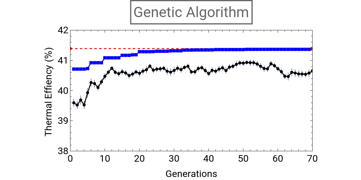
This is the genetic algorithm we coded that takes the object from the ThermodynamicCycle and returns a graphic that represents the evolution of scpecies at each generation in the horizontal axis. Also, in the vertical axis we have the Thermal Efficiency. The black line represents the mean of individuals and the blue line the best parameter of current generation. The dashed red Line is the known Maximum thermal Efficinecy.
In[]:=
In[]:=
AbsoluteTiming[AGRubel[{"NumberIndividuals"20,"ProbabilityCrossOver"0.8,"ProbabilityMutations"0.04}]]
Out[]=
30.489,