Given a set of points , the basic algorithm is 1) compute the convex hull of , 2) use the convex hull to get the GeoDelaunay mesh, compute the dual of the GeoDelaunay mesh to get the GeoVoronoi mesh.
P
P
GeoDelaunay
GeoDelaunay
We start by generating some random points on the Earth:
In[]:=
ps=Thread[RandomGeoPosition[10]]
Out[]=
{GeoPosition[{-70.0777,102.715}],GeoPosition[{-3.11357,-170.877}],GeoPosition[{-52.1682,128.301}],GeoPosition[{9.3556,150.199}],GeoPosition[{36.5912,76.9995}],GeoPosition[{-50.4875,0.627121}],GeoPosition[{25.129,-66.9782}],GeoPosition[{26.6378,128.08}],GeoPosition[{17.8991,73.9706}],GeoPosition[{26.4755,-104.142}]}
In[]:=
GeoListPlot[ps,GeoRange"World"]
Out[]=
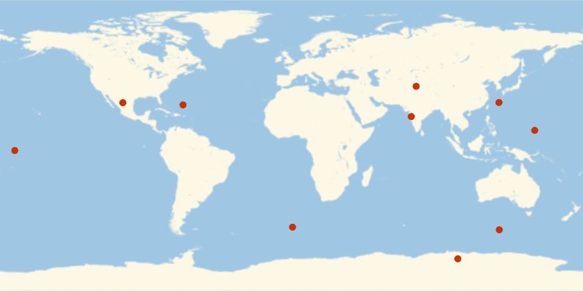
We can then compute these GeoPositions into 3D coordinates using GeoPositionXYZ:
In[]:=
Graphics3D{Red,PointSize[Large],Point[GeoPositionXYZ[ps][[1]]]},
Out[]=

ConvexHullMesh can take these 3D points and give us a mesh whose edges correspond to the edges of the GeoDelaunay mesh:
In[]:=
ConvexHullMesh[GeoPositionXYZ[ps][[1]]]
Out[]=

However, we don’t want the full convex hull but just the “outer hull” (a bit like the upper/lower hull). For example, if we have many nearby points, then the convex hull will have edges that go around the back, which we don’t want:
In[]:=
ConvexHullMeshGeoPositionXYZ["Position"][[1]]

Out[]=

By adding before computing the convex hull, we can get rid of these extra edges:
{0,0,0}
In[]:=
ConvexHullMeshAppendGeoPositionXYZ["Position"][[1]],{0,0,0}
Out[]=

We will therefore add before taking the convex hull, and then we will delete any simplices adjacent to before continuing. (Thanks to Rich Hennigan for identifying this problem and the fix). We then use MeshCells to extract the faces and generate the appropriate GeoPolygons:
{0,0,0}
{0,0,0}
In[]:=
Module[{chm,cells},chm=ConvexHullMesh[Append[GeoPositionXYZ[ps][[1]],{0.,0.,0.}]];cells=MeshCells[chm,2];If[Last[MeshCoordinates[chm]]==={0.,0.,0.},cells=Select[cells,FreeQ[MeshCellCount[chm,0]]]];GeoPolygon[Thread[ps][[#]]]&/@cells[[All,1]]]
Out[]=
{GeoPolygon[{GeoPosition[{9.3556,150.199}],GeoPosition[{-52.1682,128.301}],GeoPosition[{-3.11357,-170.877}]}],GeoPolygon[{GeoPosition[{-70.0777,102.715}],GeoPosition[{17.8991,73.9706}],GeoPosition[{-50.4875,0.627121}]}],GeoPolygon[{GeoPosition[{-70.0777,102.715}],GeoPosition[{-52.1682,128.301}],GeoPosition[{17.8991,73.9706}]}],GeoPolygon[{GeoPosition[{-52.1682,128.301}],GeoPosition[{-70.0777,102.715}],GeoPosition[{-3.11357,-170.877}]}],GeoPolygon[{GeoPosition[{-70.0777,102.715}],GeoPosition[{26.4755,-104.142}],GeoPosition[{-3.11357,-170.877}]}],GeoPolygon[{GeoPosition[{26.4755,-104.142}],GeoPosition[{-70.0777,102.715}],GeoPosition[{-50.4875,0.627121}]}],GeoPolygon[{GeoPosition[{25.129,-66.9782}],GeoPosition[{26.4755,-104.142}],GeoPosition[{-50.4875,0.627121}]}],GeoPolygon[{GeoPosition[{25.129,-66.9782}],GeoPosition[{36.5912,76.9995}],GeoPosition[{26.4755,-104.142}]}],GeoPolygon[{GeoPosition[{17.8991,73.9706}],GeoPosition[{25.129,-66.9782}],GeoPosition[{-50.4875,0.627121}]}],GeoPolygon[{GeoPosition[{36.5912,76.9995}],GeoPosition[{25.129,-66.9782}],GeoPosition[{17.8991,73.9706}]}],GeoPolygon[{GeoPosition[{-52.1682,128.301}],GeoPosition[{26.6378,128.08}],GeoPosition[{17.8991,73.9706}]}],GeoPolygon[{GeoPosition[{9.3556,150.199}],GeoPosition[{26.6378,128.08}],GeoPosition[{-52.1682,128.301}]}],GeoPolygon[{GeoPosition[{26.6378,128.08}],GeoPosition[{36.5912,76.9995}],GeoPosition[{17.8991,73.9706}]}],GeoPolygon[{GeoPosition[{36.5912,76.9995}],GeoPosition[{26.6378,128.08}],GeoPosition[{26.4755,-104.142}]}],GeoPolygon[{GeoPosition[{26.4755,-104.142}],GeoPosition[{26.6378,128.08}],GeoPosition[{-3.11357,-170.877}]}],GeoPolygon[{GeoPosition[{26.6378,128.08}],GeoPosition[{9.3556,150.199}],GeoPosition[{-3.11357,-170.877}]}]}
Packaging this into a function we get:
In[]:=
GeoDelaunay[ps_]:=Module[{chm,cells},chm=ConvexHullMesh[Append[GeoPositionXYZ[ps][[1]],{0.,0.,0.}]];cells=MeshCells[chm,2];If[Last[MeshCoordinates[chm]]==={0.,0.,0.},cells=Select[cells,FreeQ[MeshCellCount[chm,0]]]];GeoPolygon[Thread[ps][[#]]]&/@cells[[All,1]]]GeoDelaunay[ps_GeoPosition]:=GeoDelaunay[Thread[ps]]
Here are some visualizations of the results:
In[]:=
GeoGraphics[{{GeoStyling[Opacity[0.6]],RandomColor[],#}&/@GeoDelaunay[ps],Red,PointSize[Large],Point[ps]},GeoRange"World"]
Out[]=
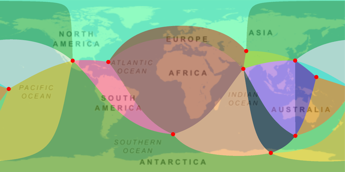
The lines look curvy because of the projection. On a globe we can see that these are geodesics:
GeoVoronoi
GeoVoronoi
The first steps in computing the GeoVoronoi are similar to those of the GeoDelaunay. We first compute the convex hull, but then we use code from here to find the vertices of the Voronoi cells:
(I tried calculating the Voronoi vertices by computing the circumcenters of the triangles using the formula here, but it gave broken results. If anyone knows why, I’d be interested to know.)
However, those GeoPositions are not necessarily on the surface of the Earth, so we will remove their altitude component:
To get the connectivity information, we could use AdjacentMeshCells to find which faces border each vertex, which correspond to the faces of the Voronoi diagram. However, AdjacentMeshCells does not preserve the ordering information. Instead, we use DualPolyhedron and extract the faces:
We use those indices to extract the GeoPositions in GeoPolygons, and package it up in a function:
We can see the relationship between the GeoVoronoi and the GeoDelaunay by plotting them together with a conformal projection. Note how corresponding edges are orthogonal:
Examples
Examples
Here we can get the Delaunay and Voronoi meshes for state capitals: