Dynamic Response of a Mercury Barometer to a Step Change in Atmospheric Pressure
Authors: Housam Binous and Ahmed Bellagi
Dynamic Response of a Mercury Barometer to a Step Change in Atmospheric Pressure
Authors: Housam Binous and Ahmed Bellagi
Authors: Housam Binous and Ahmed Bellagi
The transient dynamics of mercury rise in a barometer subjected to a sudden increase in atmospheric pressure is elucidated.
While the static equilibrium height is given by the classical hydrostatic relation ℎ=101325/(𝜌𝑔)=760mmHg, the dynamic response toward equilibrium involves fluid inertia and viscous damping effects that significantly influence the transient behavior. A momentum balance based on Newton’s second law is applied to the moving mercury column. The governing equation accounts for: Inertia of the mercury column (variable mass system), Hydrostatic restoring force due to gravity,
Height-dependent viscous friction, and Time-dependent atmospheric forcing.
To accurately capture dissipation across flow regimes, the viscous force is modeled using a Reynolds-number-based formulation. For laminar flow, Poiseuille-type resistance is used, while for turbulent flow a Blasius-type correlation is implemented (a smooth tube is assumed). This piecewise formulation enables realistic damping behavior throughout the transient process.
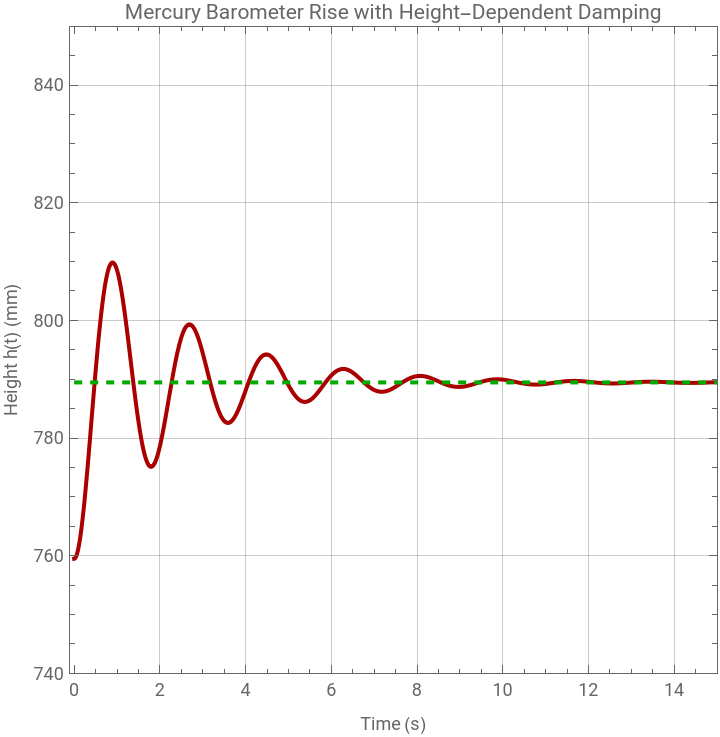
A sudden step increase in atmospheric pressure generates a rapid rise of mercury followed by a damped approach toward the new equilibrium height given by ℎ=105325/(𝜌𝑔)=789.5 mmHg.
Numerical integration using NDSolve reveals:
● A monotonic, overdamped-type response due to strong viscous effects (small tube radius),
● A final height consistent with hydrostatic theory,
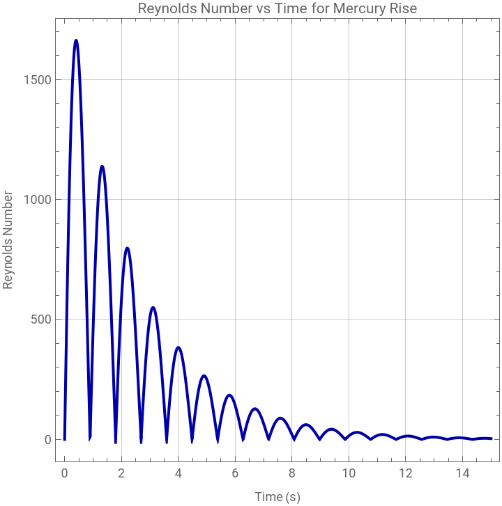
● A time-varying Reynolds number that characterizes the flow regime during the transient,
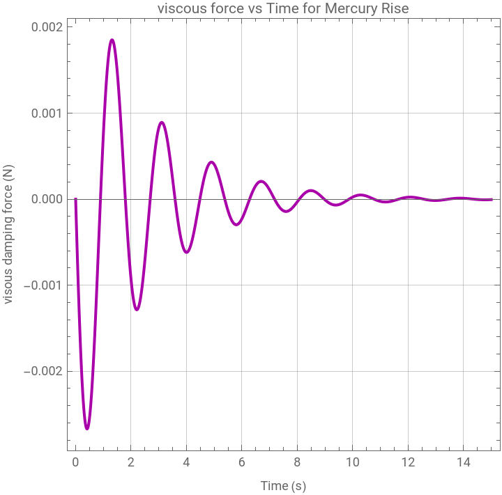
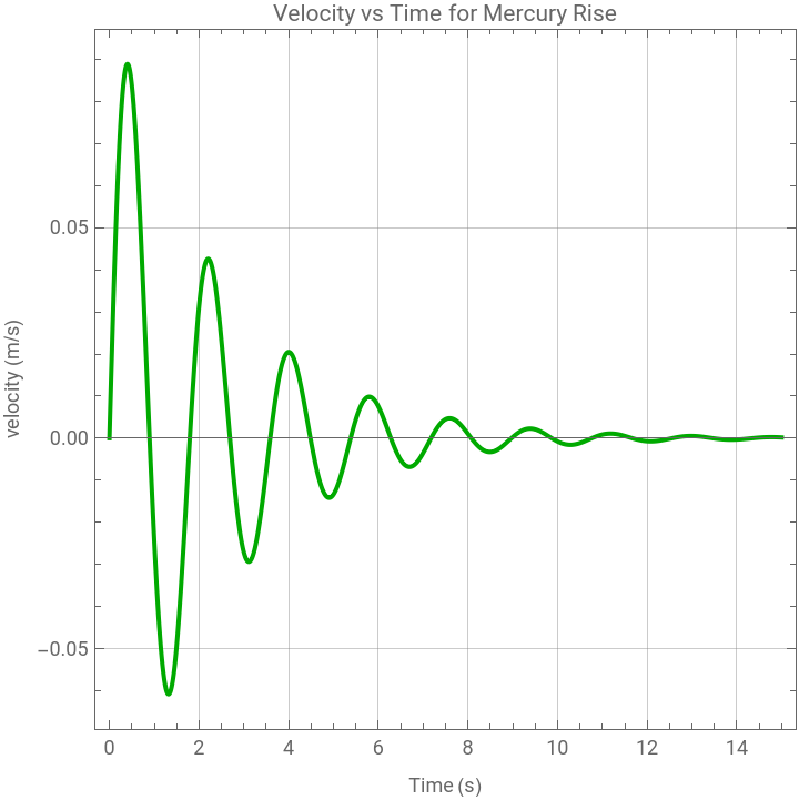
● Rapid decay of velocity and viscous force as equilibrium is approached.
The model provides insights to barometer dynamics beyond static equilibrium and illustrates how geometry and viscosity control transient behavior.
In[]:=
Reynolds[t_]:=2RrhoAbs[h'[t]]/mu
In[]:=
Ffric[t_]:=Piecewise[{{8*mu*h[t]/R^2*A*h'[t],Reynolds[t]<2000},{0.3164*Reynolds[t]^(-0.25)*rho*A*h[t]/(4*R)*h'[t]^2,Reynolds[t]>=2000}}]
In[]:=
(*governingequation---Newton'ssecondlawofmotion---height-dependentdamping*)eqn=D[Arhoh[t]h'[t],t]+Ffric[t]+gh[t]Arho==Patm[t]A
Out[]=
Agrhoh[t]+
+Arho[t]+Arhoh[t][t]APatm[t]
|
2
′
h
′′
h
In[]:=
(*fuidproperties*)rho=13600;(*Mercurydensity,kg/m^3*)mu=1.526*10^-3;(*Mercuryviscosityat20°CinPa*s)
In[]:=
g=9.81;(*Gravity,m/s^2*)
In[]:=
(*Tubeproperties*)R=1.05*10^-3;(*Tuberadius,m*)(*wepurposelytakeatubewithasmallradiusinordertoincreasedampingcoefficient*)A=PiR^2;(*Cross-sectionalarea*)
In[]:=
(*Atmosphericpressurestep*)Patm[t_]:=P0+dPUnitStep[t]P0=101325;(*atmosphericpressureinPa*)dP=4000;(*suddenpressurejump*)
In[]:=
Patm[10]
Out[]=
105325
In[]:=
(*Initialcondition:smallpositiveheighttoavoidsingularity*)ic={h[0]==P0/rho/g,h'[0]==0}
Out[]=
{h[0]0.759467,[0]0}
′
h
In[]:=
(*Solvenumericallyusingastiffsolver*)sol=NDSolve[{eqn,ic},h,{t,0,15}];
In[]:=
(*Plottransientrise*)Plot[{Evaluate[1000h[t]/.sol],1000Patm[t]/rho/g},{t,0.,15},Frame->True,AspectRatio->1,FrameLabel->{"Time (s)","Height h(t) (mm)"},PlotStyle->{{Darker@Red},{Dashed,Darker@Green}},PlotLabel->"Mercury Barometer Rise with Height-Dependent Damping",GridLines->Automatic,PlotRange->{{-0.10,15},{740,850}}]
Out[]=
In[]:=
First[h[t]/.sol/.t->15]1000(*heigthinmmHg*)
Out[]=
789.484
In[]:=
Plot[Evaluate[2RrhoAbs[h'[t]]/mu/.sol],{t,0.0,15},Frame->True,FrameLabel->{"Time (s)","Reynolds Number"},PlotLabel->"Reynolds Number vs Time for Mercury Rise",GridLines->Automatic,PlotRange->All,PlotStyle->Darker@Blue,AspectRatio->1]
Out[]=
In[]:=
Plot[Evaluate[h'[t]/.sol],{t,0.0,15},Frame->True,FrameLabel->{"Time (s)","velocity (m/s)"},PlotLabel->"Velocity vs Time for Mercury Rise",GridLines->Automatic,PlotRange->All,PlotStyle->Darker@Green,AspectRatio->1]
Out[]=
In[]:=
Plot[Evaluate[-Ffric[t]]/.sol,{t,0.0,15},Frame->True,FrameLabel->{"Time (s)","visous damping force (N)"},PlotLabel->"viscous force vs Time for Mercury Rise",GridLines->Automatic,PlotRange->All,PlotStyle->Darker@Magenta,AspectRatio->1,PlotPoints->1000]
Out[]=