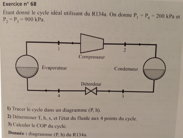
We study an ordinary vapor compression (OVC) cycle given above and reproduced from Ref. 1. The condenser pressure (high pressure) and evaporator pressure (low pressure) are 900 kPa and 200 kPa. The coefficient of performance (COP), which is the heat transferred to the evaporator divided by the compressor work, is calculated.
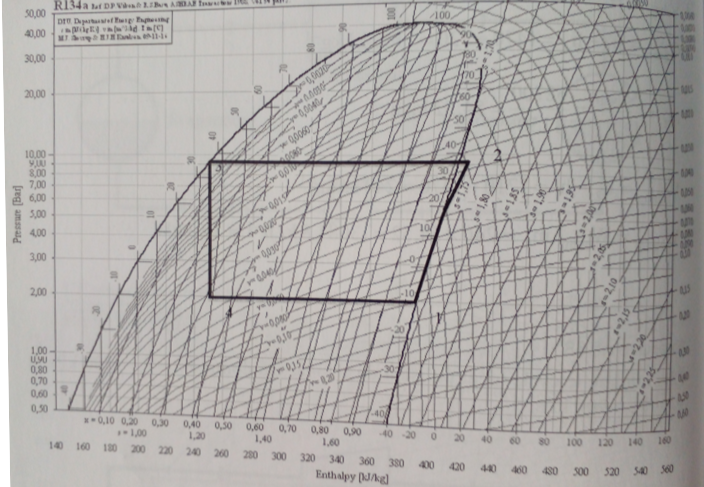
H - P data
H - P data
plh=(*{"Enthalpy (kJ/kg)","Pressure (MPa)"},*);pvh=(*{"Enthalpy (kJ/kg)","Pressure (MPa)"},*);
In[]:=
f=Interpolation[plh]
Out[]=
InterpolatingFunction


In[]:=
plt=ListLogPlot[{plh,pvh},JoinedTrue,FrameTrue,AspectRatio1,GridLinesAutomatic,FrameLabel{Style["Enthalpy (kJ/kg)",14],Style["Pressure (MPa)",14]}]
Out[]=
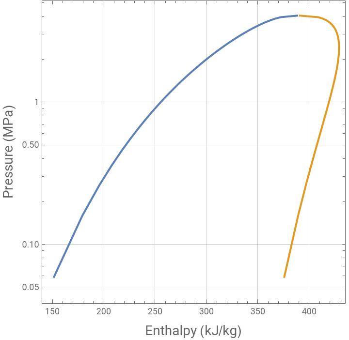
tls=(*{"Entropy (J/g*K)","Temperature (K)"},*);
tvs=(*{"Entropy (J/g*K)","Temperature (K)"},*);
In[]:=
plt2=ListPlot[{tls,tvs},JoinedTrue,FrameTrue,AspectRatio1,GridLinesAutomatic,FrameLabel{Style["Entropy (kJ/kg*K)",14],Style["Temperature (K)",14]}]
Out[]=
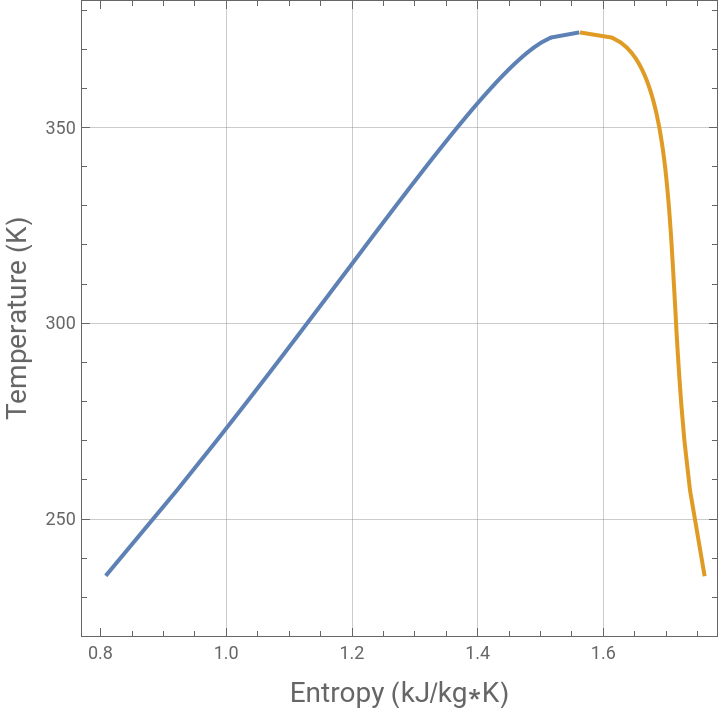
Link for R134a - TetraFlouroEthane Saturation Properties - Pressure Table Pressure Temp volume (m^3/kg) energy (kJ/kg) enthalpy (kJ/kg) entropy (kJ/kg.K) kPa deg C vf vg uf ug hf hfg hg sf sfg sg
data=;
In[]:=
delta=148.146;
In[]:=
tbl1=Table[{data[[i]][[9]]+delta,Log[data[[i]][[1]]/1000]},{i,1,Length[data]}]
Out[]=
{{375.946,-2.81341},{379.616,-2.52573},{382.606,-2.30259},{385.126,-2.12026},{387.326,-1.96611},{389.266,-1.83258},{391.026,-1.7148},{392.616,-1.60944},{394.086,-1.51413},{395.446,-1.42712},{396.706,-1.34707},{397.886,-1.27297},{398.996,-1.20397},{400.046,-1.13943},{401.036,-1.07881},{401.976,-1.02165},{403.726,-0.916291},{407.476,-0.693147},{410.576,-0.510826},{413.196,-0.356675},{415.466,-0.223144},{417.436,-0.105361},{419.166,0.},{422.046,0.182322},{424.296,0.336472},{426.046,0.470004},{427.356,0.587787},{428.286,0.693147},{429.006,0.916291},{427.336,1.09861}}
In[]:=
tbl2=Table[{data[[i]][[7]]+delta,Log[data[[i]][[1]]/1000]},{i,1,Length[data]}]
Out[]=
{{152.003,-2.81341},{159.374,-2.52573},{165.444,-2.30259},{170.653,-2.12026},{175.246,-1.96611},{179.372,-1.83258},{183.133,-1.7148},{186.598,-1.60944},{189.818,-1.51413},{192.832,-1.42712},{195.67,-1.34707},{198.355,-1.27297},{200.905,-1.20397},{203.338,-1.13943},{205.665,-1.07881},{207.897,-1.02165},{212.113,-0.916291},{221.504,-0.693147},{229.684,-0.510826},{236.995,-0.356675},{243.647,-0.223144},{249.786,-0.105361},{255.496,0.},{265.946,0.182322},{275.406,0.336472},{284.116,0.470004},{292.256,0.587787},{299.956,0.693147},{317.846,0.916291},{334.706,1.09861}}
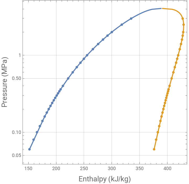
Both P-H data sets plotted on the same diagram
Both P-H data sets plotted on the same diagram
In[]:=
Show[plt,ListPlot[{tbl2,tbl1},PlotStyle{{PointSize[0.015]}}]]
Out[]=
data1=;
In[]:=
q=Table[{data1[[i]][[1]],data1[[i]][[5]]},{i,1,Length[data1]}]
Out[]=
{{35.51,0.9169},{40.,0.9327},{50.,0.966},{60.,0.9976},{70.,1.028},{80.,1.0574},{90.,1.086},{100.,1.114},{110.,1.1414},{120.,1.1684},{130.,1.1949},{140.,1.221},{150.,1.2467},{160.,1.2721},{170.,1.2972},{180.,1.3221}}
In[]:=
f6=Interpolation[q]
Out[]=
InterpolatingFunction

In[]:=
tbl3=Table[{data[[i]][[1]]/1000,data[[i]][[12]]},{i,1,Length[data]-4}]
Out[]=
{{0.06,0.96446},{0.08,0.95715},{0.1,0.95188},{0.12,0.94784},{0.14,0.94462},{0.16,0.94196},{0.18,0.93972},{0.2,0.93779},{0.22,0.93612},{0.24,0.93465},{0.26,0.93334},{0.28,0.93217},{0.3,0.9311},{0.32,0.93014},{0.34,0.92925},{0.36,0.92844},{0.4,0.92698},{0.5,0.92408},{0.6,0.92185},{0.7,0.92001},{0.8,0.91843},{0.9,0.917},{1.,0.91566},{1.2,0.91312},{1.4,0.91059},{1.6,0.90795}}
ENTROPY & TEMPERATURE @ POINT 2 is S2=1.7341 and T2=-10.076°C
POINT 2 IS SATURATED VAPOR @ P=0.2 MPa
POINT 2 IS SATURATED VAPOR @ P=0.2 MPa
ENTHALPY @ POINT 4 is H4=249.781 kJ/kg
TRANSFORMATION 4→1 IS ISENTHALPIC H1=H4=249.781 kJ/kg
TRANSFORMATION 4→1 IS ISENTHALPIC H1=H4=249.781 kJ/kg
ENTHALPY @ POINT 2 is H2=392.745 kJ/kg
ENTROPY & TEMPERATURE @ POINT 3 is S3=1.73887 and T3=323.273
TRANSFORMATION 2→3 IS ISENTROPIC hence S3=S2
TRANSFORMATION 2→3 IS ISENTROPIC hence S3=S2
ENTHALPY @ POINT 3 is H3=423.914
SUMMARY OF PRESSURES AND ENTHALPIES @ POINTS 1, 2, 3 AND 4
POINTS 1 IS IN THE TWO-PHASE REGION
LET US DETERMINE ITS QUALITY (EQUAL TO 0.3064)
LET US DETERMINE ITS QUALITY (EQUAL TO 0.3064)
The coefficient of performance is equal to 4.586
The OVC Cycle drawn on the H-P diagram
TEMPERATURE @ POINTS 1, 3 and 4
The OVC Cycle drawn on the T-S diagram
References
References
◼
[1] D. Ronze, Coordonnateur, Introduction au génie des procédés: Applications et développements, Tec & Doc, Paris, Lavosier, 2013.
CITE THIS NOTEBOOK
CITE THIS NOTEBOOK
Ideal cycle using R134a
by Housam Binous
Wolfram Community, STAFF PICKS, January 18, 2025
https://community.wolfram.com/groups/-/m/t/3359290
by Housam Binous
Wolfram Community, STAFF PICKS, January 18, 2025
https://community.wolfram.com/groups/-/m/t/3359290