Terminal Fall Velocity in Newtonian and Power-Law fluids
Authors: Housam Binous and Ahmed Bellagi
Terminal Fall Velocity in Newtonian and Power-Law fluids
Authors: Housam Binous and Ahmed Bellagi
Authors: Housam Binous and Ahmed Bellagi
Terminal fall velocity in Newtonian fluids at low Reynolds numbers
In[]:=
g=9.81;(*m/s^2*)rhoS=7800;(*spheredensitykg/m^3*)rhoF=1260;(*glycerindensityat20°Cinkg/m^3*)mu=1.49;(*glycerinviscosityat20°CinPa.s*)r=1*10^-3;(*sphereradiusm*)(*spherevolume*)volume=(4/3)Pir^3;(*massofsphere*)m=rhoSvolume;(*Newton'ssecondlawofmotion*)eqn=v'[t]==(mg-rhoFvolumeg-6Pimurv[t])/m;ic=v[0]==0;(*initiallythesphereisatrest*)sol=NDSolve[{eqn,ic},v,{t,0,5}];(*TerminalfallvelocitybasedonStokes'law*)vTerminal=(2r^2g(rhoS-rhoF))/(9mu);(*plotofvelocityversustime*)Plot[{Evaluate[v[t]/.sol],vTerminal},{t,0,0.01},PlotStyle->{Darker@Blue,{Darker@Red,Dashed}},PlotLegends->{"Numerical velocity","Theoretical v_t"},FrameLabel->{"t (s)","v (m/s)"},GridLines->Automatic,PlotRange->All,AspectRatio->1,Frame->True]
Out[]=
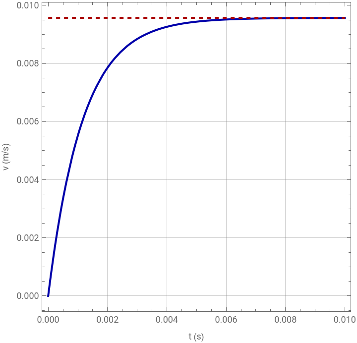


In[]:=
(*CheckReynoldsnumberisindeedlessthan1*)Reynolds=rhoFvTerminalDs/mu/.Ds->2r
Out[]=
0.0161831
In[]:=
Plot[Evaluate[v'[t]/.sol],{t,0,0.01},PlotStyle->Darker@Green,PlotLabel->"Numerical acceleration",FrameLabel->{"t (s)","v' (m/s^2)"},GridLines->Automatic,PlotRange->All,AspectRatio->1,Frame->True](*asthevelocityincreasesfromzerototheterminaalfallvelocity,thedragincreasesuntilitequatesthenetweightandtheaccelerationbecomesnil*)
Out[]=
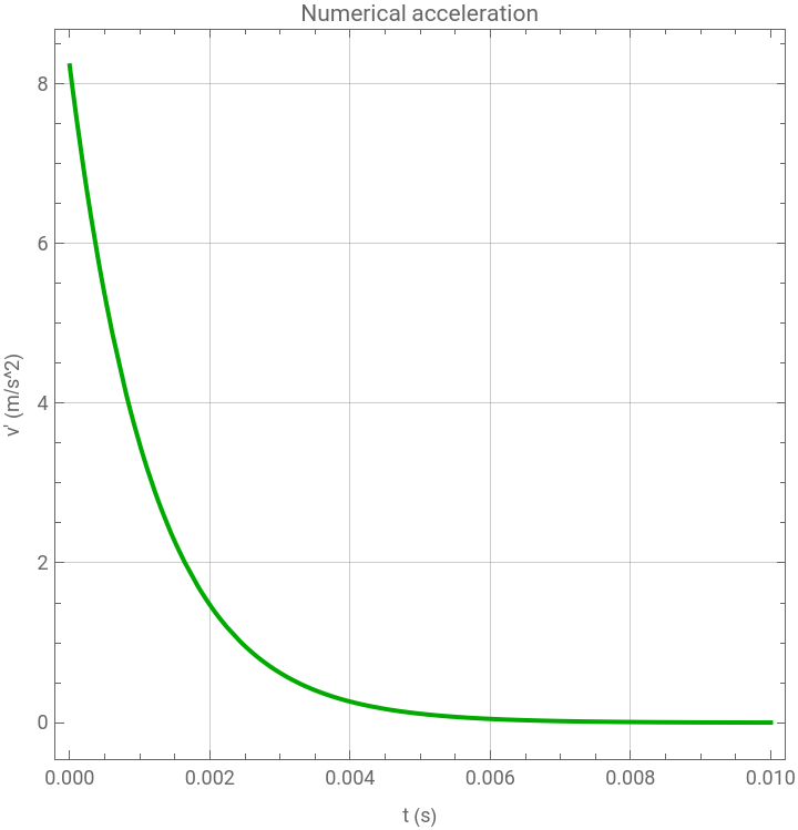
Effect of temperature on the terminal fall velocity
(*glycerinviscosityversustemperaturedatafromDOI:
10.1007/s00348-012-1432-z
*)data={{20,1.48},{40,0.330},{60,0.102},{80,0.035},{100,0.013}};In[]:=
nlm=NonlinearModelFit[data,aExp[-b(T-20)],{a,b},T]
Out[]=
FittedModel
(*Viscositymodel*)muGlycerin[T_]:=Normal[nlm]
In[]:=
Show[Plot[muGlycerin[T],{T,15,105},FrameLabel->{"Temperature","viscosity"},Frame->True,PlotRange->All,GridLines->Automatic,PlotStyle->Darker@Blue,AspectRatio->1],ListPlot[data,PlotStyle->{PointSize[0.02],Darker@Red}]]
Out[]=
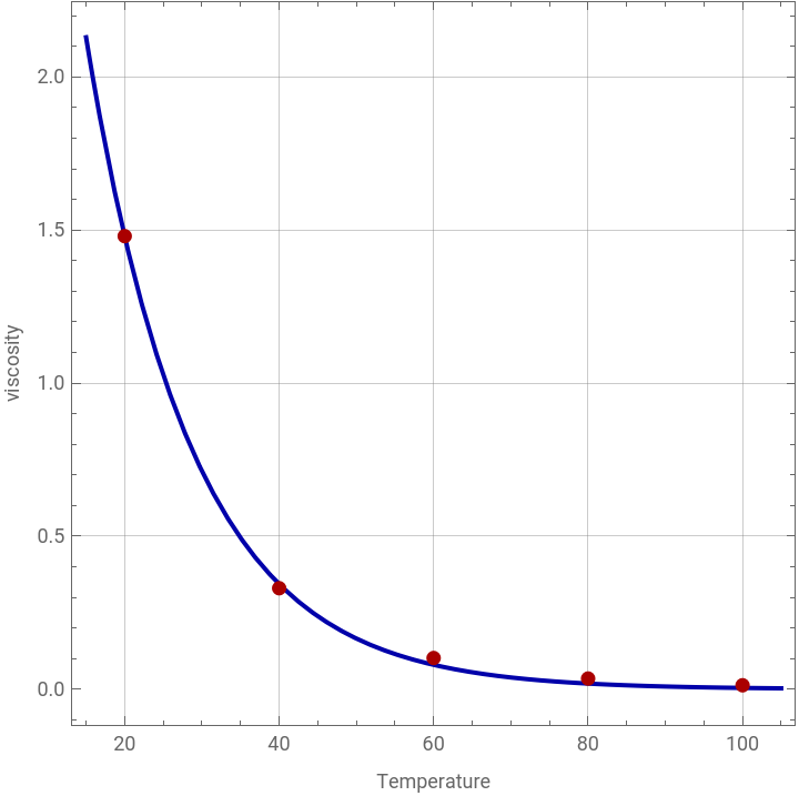
In[]:=
(*Terminalvelocityvstemperature--weassumeethatrhoFisconstant(i.e.,independantofT)*)vT[T_]:=(2r^2g(rhoS-rhoF))/(9muGlycerin[T]);Plot[vT[T],{T,20,50},FrameLabel->{"Temperature (°C)","Terminal velocity (m/s)"},GridLines->Automatic,PlotRange->All,AspectRatio->1,Frame->True,PlotStyle->Darker@Magenta](*forlargetemperatures,thevelocityislargersinceviscosityofthefluiddecreases*)
Out[]=
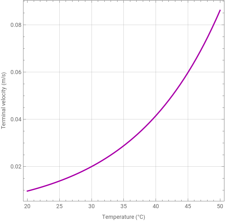
Terminal fall velocity in non-Newtonian fluids at low Reynolds numbers
In[]:=
(*Constants*)g=9.81;r=1*10^-3;rhoS=7800;rhoF=1000;(*Power-lawparameters*)K=0.8;(*Pa.s^n*)n=0.6;(*shear-thinningfluid*)(*volume*)volume=(4/3)Pir^3;(*mass*)m=rhoSvolume;Fg=mg;(*downwardweight*)Fb=rhoFvolumeg;(*upwardbuoyantforce*)Cd=6PiKr^(2-n);(*dragcoefficient*)(*governingequationandinitialcondition*)eqn=v'[t]==(Fg-Fb-Cdv[t]^n)/m;ic=v[0]==0;sol=NDSolve[{eqn,ic},v,{t,0,5}];(*Terminalvelocity*)vTerminal=((Fg-Fb)/Cd)^(1/n);(*Plot*)Plot[{Evaluate[v[t]/.sol],vTerminal},{t,0,0.15},PlotStyle->{Darker@Blue,{Darker@Red,Dashed}},PlotLegends->{"Numerical velocity","Terminal velocity"},FrameLabel->{"t (s)","v (m/s)"},GridLines->Automatic,PlotRange->All,AspectRatio->1,Frame->True]