Cellular automata, or CA, are models that consist of a grid of cells, each of which can be in a finite number of states. These cells evolve over discrete time steps according to a set of rules based on the states of neighboring cells. They are used to simulate complex systems in various fields, including mathematics, physics, and computer science, and have recently been applied in modeling genome. In this study, our focus is a CA rule that can be used for optimized horizontal expansion in genomic modeling, such as cells turning into infinity or similar-entropy twin rules.
Introduction
Introduction
In his article “Foundations of Biological Evolution: More Results & More Surprises,” Stephen Wolfram used cellular automata to model genomic evolution under the fitness criterion of “live as long as possible but die eventually [1].” This criterion emphasized durability and longevity over horizontal expansion. In contrast, our study seeks to identify and interpret the rule that optimizes horizontal expansion - favoring chain mutations and the emergence of increased randomness - while still ensuring that the organism eventually dies in order to maintain a realistic and natural evolutionary constraint.
This alternative criterion fosters an environment in which genetic mutations are more frequent, a condition we hypothesize may enhance an organism’s ability to spread across space. We believe that the most efficient pattern for such expansion may resemble a pyramid, and our experiments aim to verify or refute this through empirical simulation and theoretical reasoning.
To achieve this, we mathematically analyze rule behaviors by computing parameters such as entropy and density, enabling us to fabricate an optimal rule function for horizontal expansion. Finally, we explore a critical edge case: rules that are initially finite but become infinite due to point mutations. Unlike boundary-dependent growth, these cases suggest an emergent form of infinite behavior, challenging assumptions about fixed rule outcomes.
Rule determination
Rule determination
In the first stage of the project, the goal is to identify cellular automata rules that exhibit finite horizontal expansion - spreading across space for a period before stabilizing or dying out. This form of controlled, self-limiting growth is ideal for modeling biological phenomena such as gene expression waves or tissue growth boundaries, where expansion is guided by internal dynamics rather than infinite propagation.
Rules are systematically tested, and those that demonstrate both non-trivial spatial spread and eventual extinction are selected for deeper analysis. By comparing the dynamics of these candidate rules, we begin to recognize behaviors that more closely simulate genome-like processes.
Rules are systematically tested, and those that demonstrate both non-trivial spatial spread and eventual extinction are selected for deeper analysis. By comparing the dynamics of these candidate rules, we begin to recognize behaviors that more closely simulate genome-like processes.
Triplets count
Triplets count
To start, we need to find the best rule for the expansion goal. In Cryptography with Cellular Automata, rule 30 was introduced as a rule with high entropy, which made it a good fit for cryptography [2]. However, that does not ensure its validity for genomic representation. As a result, we test rules based on different types of randomness and other parameters to determine their fitness.
To test those rules, the function usedRuleCasesFixed, was identified to simulate a cellular automaton starting from a fixed initial condition—a single black cell centered in an otherwise white array—and evolves it for a given number of steps. It then counts how many unique 3-cell neighborhoods (triplets) appear throughout the evolution, reflecting the diversity of local patterns generated by the rule.
In[]:=
usedRuleCasesFixed[rule_Integer,steps_Integer:100,initLength_Integer:101]:=Module[{evolution,triplets},evolution=CellularAutomaton[rule,ReplacePart[ConstantArray[0,initLength],Ceiling[initLength/2]->1],steps];triplets=Flatten[Partition[PadLeft[#,initLength+2,0],3,1]&/@evolution,1];Length@DeleteDuplicates[triplets]]
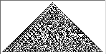
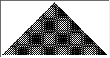
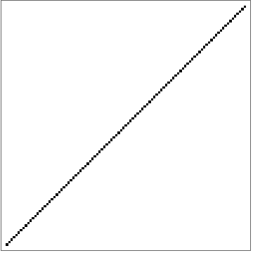
Then, we test different rules known for randomness or - in contrast - regularity. For example on a 100-step scale, the rule 30 scored a perfect 8/8. However, this perfection was matched by other rules such as rule 190, so by lowering the number of steps to 2 - as most rules are known for irregular starts, rule 190 showed more promising values. In contrast, rule 10 which is known for being regular showed a low score of 4/8.
In[]:=
usedRuleCasesFixed[30,100]usedRuleCasesFixed[30,2]
Out[]=
8
Out[]=
7
In[]:=
usedRuleCasesFixed[190,100]usedRuleCasesFixed[190,2]
Out[]=
8
Out[]=
8
In[]:=
usedRuleCasesFixed[10,100]usedRuleCasesFixed[10,2]
Out[]=
4
Out[]=
4
The visual representation of their cellular automata further highlights the difference.
From left to right: rule 30, rule 190, and rule 10.
In[]:=
Row[{ArrayPlot[CellularAutomaton[30,{{1},0},100],ImageSize->Small],ArrayPlot[CellularAutomaton[190,{{1},0},100],ImageSize->Small],ArrayPlot[CellularAutomaton[10,{{1},0},100],ImageSize->Small]}]
Out[]=
Testing the chance of mutations
Testing the chance of mutations
In biological environments, genetic mutations can sometimes be an evolutionary rescue during environmental changes. Members with genetic mutations have a chance of surviving the change and passing their characteristics down to their lineage, which makes the chance of a mutation occurring in any genetic modelling a must. Mutations’ chance testing is the second step in our rule determination process, for better expansion and real-life simulation.
The function mutateOneBit takes an 8-bit integer representing a rule, flips one randomly chosen bit, and returns the resulting integer—effectively introducing a small mutation.
In[]:=
mutateOneBit[rule_Integer]:=Module[{bits,idx},bits=IntegerDigits[rule,2,8];idx=RandomInteger[{1,8}];bits[[idx]]=1-bits[[idx]];FromDigits[bits,2]];
The function hillClimbGenomeExpansion goes through the rules, updating the output whenever a rule scores a better score when compared to its predecessor.
In[]:=
hillClimbGenomeExpansion[initRule_Integer,stepsPerEval_Integer:100,initLength_Integer:101,gens_Integer:500]:=Module[{current=initRule,bestScore,newRule,newScore},bestScore=usedRuleCasesFixed[current,stepsPerEval,initLength];Table[newRule=mutateOneBit[current];newScore=usedRuleCasesFixed[newRule,stepsPerEval,initLength];If[newScore>=bestScore,current=newRule;bestScore=newScore;{"Gen ",gen,": rule=",current," score=",bestScore};],{gen,1,gens}];{current,bestScore}]
As we see below, we tested a group of random rules, taking only the better results to decrease the number of sampled rules.
In[]:=
{bestRule,bestScore}=hillClimbGenomeExpansion[RandomInteger[{0,255}],100,101,300];
Table[{r,usedRuleCasesFixed[r,100,101]},{r,{30,45,90,106,bestRule}}]
Out[]=
{{30,8},{45,8},{90,8},{106,4},{92,8}}
The helper function usedRuleCasesSeeded computes the number of unique triplets encountered over time by padding and partitioning each step of the automaton’s evolution.
In[]:=
usedRuleCasesFixedSeeded[rule_,steps_,seed_]:=Module[{evolution,triplets,usedTriplets,initLength=Length[seed]},evolution=CellularAutomaton[rule,seed,steps];triplets=Flatten[Table[Partition[PadLeft[evolution[[t]],initLength+2,0],3,1],{t,1,Length[evolution]}],1];usedTriplets=DeleteDuplicates[triplets];Length[usedTriplets]];
The function evaluateWithRandomSeeds runs a cellular automaton rule multiple times with random initial seeds, evaluates how many unique 3-cell patterns (triplets) are used during evolution, and returns the average across all runs.
In[]:=
evaluateWithRandomSeeds[rule_,numSeeds_:10,steps_:100,initLength_:101]:=Module[{scores},scores=Table[Module[{seed},seed=RandomInteger[{0,1},initLength];usedRuleCasesFixedSeeded[rule,steps,seed]],{numSeeds}];Mean[scores]];
Additional factors testing: Novelty, Entropy & Branching
Additional factors testing: Novelty, Entropy & Branching
As we see below, despite the filtration, there are still a lot of rules that achieve a perfect 8/8 score, which leads us to test the following parameters: Novelty score (How much novelty grows over time), Entropy, and Branching score.
Novelty score is not just about randomness and uniqueness on a cell-to-cell basis. It’s more of how this uniqueness keeps growing over time so that the cell does not end up settling on one defined pattern after some point in time. Entropy, specifically Shannon entropy is best described as the cell-to-cell randomness. The branching score is the reproduction rate of each cell, and in expansion cases, the greater the branching score, the more diverse the model, and the better results you gain.
Novelty score is not just about randomness and uniqueness on a cell-to-cell basis. It’s more of how this uniqueness keeps growing over time so that the cell does not end up settling on one defined pattern after some point in time. Entropy, specifically Shannon entropy is best described as the cell-to-cell randomness. The branching score is the reproduction rate of each cell, and in expansion cases, the greater the branching score, the more diverse the model, and the better results you gain.
The function tripletUsageOverTime computes the number of triplets each rule uses with respect to the time factor.
The function stateEntropy computes the entropy of the system’s states.
The function branchingScore measures divergence in behavior.
The function tripletUsageOverTime computes the growth in unique triplets over time.
The function evaluateFitness computes a composite fitness score for a cellular automaton rule by combining the three metrics: the growth in unique triplets over time, the entropy of the system’s states, and a branching score that measures divergence in behavior.
Finally, we sort the rules based on how high they scored in the evaluating fitness test, to get the best rule.
In conclusion, rule 178 gets the highest score of 256.296. That score makes rule 178 the optimal rule for genome expansion according to our testing.
Rule 178: General pattern randomness
Rule 178: General pattern randomness
As shown, the most optimal rule identified through our tests is Rule 178, selected based on multiple criteria relevant to genomic modeling. The form of randomness exhibited by Rule 178 differs notably from that of Rule 30. While Rule 30 produces randomness at the cell-to-cell level, appearing chaotic and patternless, Rule 178 exhibits structured variability—switching between sets of recognizable, repeating patterns. This balance between order and randomness makes Rule 178 particularly suitable for modeling biological processes that require both stability and adaptability.
Visual representation of rule 178, the most optimal rule for genome expansion.
Rule 178 stands out due to its pattern of “clustered randomness”—structured regions that shift or repeat unpredictably, resembling regulatory behavior in real genomic systems. In contrast, rule 95 shows linear, deterministic expansion, yet both rules share nearly identical entropy levels, which may be useful for our work later on. We will be referring to rule 95 as rule 178’s “linear twin.” This investigation highlights how entropy alone does not reflect the complexity or modeling potential of a rule, that’s why it’s combined with other parameters like branching score, continuous novelty, etc.
The entropy of rules 30, 178, and 95 respectively.
This result suggests that Rule 178 achieves greater long-term unpredictability while still preserving coherent structures - a crucial property for modeling genetic systems where mutations must be both diverse and biologically viable. Its consistent transition behavior, high entropy, and rich pattern dynamics make Rule 178 an ideal rule for simulating mutation-driven evolution in cellular automata and artificial life systems.
A closer look at the resulting mutations
A closer look at the resulting mutations
We notice that rule 178 is dealing with a deeper level of mutations even with the same parameters, which leads to some sort of increased mutating sample. As a consequence, the probability for a mutation increases which explains the high entropy.
In the start, we checked the 2-color range-2 totalistic code of rules 178 and 30’s cellular automata from a sequence of initial conditions.
The result is a perfect pyramid pattern - highly symmetric and expanding linearly in both directions. This is called pyramidal growth in 1D CA - a sign of an orderly but expanding structure. The pyramid shape means each new row is wider, so the genome “expands” predictably and consistently.
This plot shows how Rule 178 evolves from a single cell over 200 steps
This output {2, 3, 3, 4, 4, 5, ...} shows that as n increases, the CA takes longer to stabilize. This result suggests Rule 178 has increasing complexity with larger genomes — which aligns with evolutionary potential. The test confirms that Rule 178 avoids predictable repetition and keeps evolving longer with size.
This code computes how many steps it takes until a pattern with n cells stabilizes or repeats
The following visualisation reveals multiple attractors - distinct cycles that different initial configurations evolve into—highlighting its structured yet diverse behavior. This property makes rule 178 a compelling model for studying gene mutations, where different genetic sequences (initial states) may stabilize into various expression patterns (attractors). The presence of multiple basins of attraction mirrors how mutations can lead to different phenotypic outcomes, some stable and others transient.
The state transition graph of Rule 178 over 7-bit strings
Here we visualise how small changes in input affect output, like mutating a genome slightly and watching the effect. The transition graph shows a checkered diamond pattern — which means Rule 178 reacts predictably and symmetrically to perturbation. This property makes it robust yet still unpredictable in the long run.
A look at the inner pattern of rule 178
A zoomed-in look at the 3D modeling of Rule 178 versus Rule 30 reveals interesting differences in the structure and scale of randomness. Although both rules produce triangular growth when viewed in one dimension, Rule 30 exhibits local, high-frequency variation, while Rule 178 appears more uniform and predictable at first glance. This pattern is evident from the perturbation plot, where Rule 178 responds symmetrically to small changes in initial conditions. Mathematically, this behaviour suggests low local entropy and low sensitivity to initial conditions—properties often associated with Class 2 behavior in Wolfram’s classification - that refers to cellular automata where the development of all patterns tends toward simple stationary states. However, this behaviour changes in the global 3D representation: the number of active states (cells with value 1) in Rule 178, plotted across time and space, grows with a denser and more nonlinear distribution than initially expected. Over a time series 𝑡, the number of unique spatial configurations observed in Rule 178 scales faster than in Rule 30. That is, while Rule 30 maximizes Shannon entropy in short sequences, Rule 178 yields a higher Kolmogorov complexity over longer time intervals.
- Shannon entropy, often denoted as H(X), is defined for a discrete random variable X with possible outcomes x1, x2, x3,.....xn and corresponding probabilities p(x1), p(x2), p(x3),..., p(xn).
- Kolmogorov complexity is a measure of the computational resources needed to specify the object and is also referred to as Solomonoff–Kolmogorov–Chaitin complexity, program-size complexity, descriptive complexity, or algorithmic entropy.
Additionally, when we viewed both rules (as range-2, two-color totalistic cellular automata) across a sequence of initial conditions, we observed that Rule 178 introduces structural variability with smaller perturbations, often hidden in 1D due to the compactness of its short-term behavior. Yet in 3D, these minor differences compound, and the space of active states begins to resemble a branching structure — similar to cumulative mutations in evolving genomes.
In the context of genetic modeling, this distinction is critical. Evolutionary dynamics often hinge not on local randomness but on global variability—how the system behaves over many generations. From this perspective, Rule 178’s behavior demonstrates emergent complexity that better reflects genome expansion and long-term evolve-ability. Hence, while Rule 30 may appear more chaotic in local metrics, Rule 178 exhibits deeper randomness over time, making it a more biologically plausible candidate for modeling genetic evolution.
3D representation of rules 178 and 30, respectively
Application: Comparing mutations in CA with cancer colonies
Application: Comparing mutations in CA with cancer colonies
While Rule 178 appears predictable in 1D, its 3D evolution reveals a broader, more irregular expansion—one that resembles patterns seen in early cancer proliferation. By analyzing how the width of active cells increases over time, we can draw parallels between the automaton’s spreading front and the spatial growth of tumor tissue. In both systems, localized changes (mutations or perturbations) can accumulate to produce globally significant outcomes, making Rule 178 a useful minimal model for studying long-run expansion in biological systems.
Quite similar in logic to function tripletUsageOverTime that was mentioned before, function widthOverTimeData measures the horizontal expansion of a simulated rule with respect to time.
Preparing the width over time data for both rules 178 and 30 for a valid comparison.
The Gompertz growth model is a mathematical model used to describe the growth dynamics of tumours. It closely mimics the actual growth patterns of many tumors, making it a critical tool in both theoretical biology and medical research. Currently, we will be using it to mathematically model early-stage tumours during proliferation stage.
Finally, we can plot the comparison between the three expansion models.
The line graph above showed how the three models expand. However rule 178 shows more sturdy expansion, even though it’s changing, which mimics tumour growth better - specifically Gompertz model. The stability point is almost the same for the three models, however the difference lies in the rate of expansion before this point varies among the different models.
Rule 178 in 3D modelling
Rule 178 in 3D modelling
When we visualize rule 178 and rule 30 in 3D, we notice how this allowed us different perspectives on how certain rules exhibit certain characteristics, e.g.; randomness, regularity, connectivity, or linearity. This angle takes us to a new chapter on cellular automata in 3D, and how important it is to consider all the parameters in multidimensional forms when dealing with cellular automaton rules - especially in genome visualization.
Density
Density
Density is one of the most crucial aspects of 3D bodies that is often overlooked when working on genome representation. However, when discussing genome “expansion,” density and related parameters - such as infill percentage and connectivity functions - are important for understanding whether an organism is truly “expanding.” Additionally, the strength of connections, their proximity, and the density of each point are all key measures of this expansion.
As a starter, infill percentage should be identified, which is the ratio of filled cells of the slice over the overall volume of the 3D model. It represents one of the cornerstones in measuring density, as it determines the relation between filament and air inside the object.
This function was first introduced in “Cellular automata generation of 3D printer infill.”
The evolution here represents the cellular automaton of rule 178, which we need for the density testing later on.
Then we define the 3D representation of the binary cellular automaton, as the infill percentage is a property exclusive for 3D bodies.
Finally, the infill percentage of the 3D body is defined, which we need for the density calculation in the next step.
Another parameter is connectivity which is the degree to which cells in the structure are interconnected. A higher connectivity accompanied with a greater lifetime width indicates a denser environment and a more significant expansion.
The function ComponentMeasurments is used as a measure of objects’ connectivity.
Then, both parameters are connected to derive the density, which is the infill percentage multiplied by the reciprocal of the component measurement - which is the amount of connected components of the body. In other words, it’s the amount of filled dots over the overall dots in a connected pattern.
The density of the CA is defined as infill percentage x 1/connectivity
Finally, we can plot the density and check if our supposed expansion is dense enough for a decent level of genomic diversity.
As always, we need to plot the 3D data first for all properties that are exclusive to 3D bodies
ListInterpolation is used to represent an approximate function that interpolates the array of values given.
Finally we plot the density, which appears to be evenly distributed along the cubic body.
Rule 178 demonstrates a relatively regular density distribution across the cellular automaton grid, reflecting a pattern of widespread but sparse activity. This even spread aligns to support horizontal expansion through chain mutations, as it avoids clustering and allows mutations to propagate broadly. Thus, Rule 178’s density characteristics make it a compelling candidate for modeling genomic expansion patterns consistent with the study’s objectives.
We repeat the same process as in our last density representation, but now for rule 30.
In the end, we compute the density of rule 30 to compare it with rule 178.
Rules 30 and 178 have the same overall density but Rule 178 achieves it with fewer active cells. This observation means Rule 178’s active cells are more concentrated or efficient in spreading mutations within a limited space. Rule 30, by contrast, spreads its activity over a larger area, possibly creating more randomness but less spatial efficiency. For genome modeling focused on horizontal expansion, Rule 178’s ability to maintain density with fewer cells represents more targeted, compact mutation chains, while Rule 30 might simulate broader, more chaotic expansions.
Conclusion
Conclusion
In conclusion, this study provides a comprehensive framework for exploring cellular automaton rules as representatives to genomic behavior. By shifting focus from pure longevity to horizontal expansion followed by finite death, we simulate mutation-rich environments more aligned with early evolutionary stages. Rule 178, with its pyramid growth and structured randomness, stands out as a strong candidate for representing such environments. Meanwhile, the emergence of rule 95 and its hybrids show that directional flow and decentralization also play important roles in expansion efficiency.
The hybridization of rules—mathematically and behaviorally—demonstrates that entropy alone is not enough. The balance between density, connectivity, and local novelty gives a better indicator of evolutionary potential. Finally, by experimenting with point mutations and tracking transitions from finite to infinite behavior, we open the door to simulating sudden shifts in genetic expression, like those seen in tumorous growth. This multi-angle approach, combining symbolic logic, visual evolution, and statistical modeling, builds a more biologically intuitive understanding of cellular automata in genomic simulation.
The hybridization of rules—mathematically and behaviorally—demonstrates that entropy alone is not enough. The balance between density, connectivity, and local novelty gives a better indicator of evolutionary potential. Finally, by experimenting with point mutations and tracking transitions from finite to infinite behavior, we open the door to simulating sudden shifts in genetic expression, like those seen in tumorous growth. This multi-angle approach, combining symbolic logic, visual evolution, and statistical modeling, builds a more biologically intuitive understanding of cellular automata in genomic simulation.
Future work
Future work
1) Rule hybridization opens the way to cross-over simulation, which can mimic sexual reproduction and along with occasional point mutations can be used to get more realistic in-depth genomic mutation.
2) Finite-rules-turning-infinite mutations can be applied in medical and pathological studies, like cell regeneration and the treatment of degenerative retinal cells.
3) On the other hand, further studies on mutating infinite rules until they turn infinite can be suitable representations of genetic treatments of cancerous cells or tumours.
4) The rules that were analysed in this study, e.g., rule 178, rule 95, rule 30, can be used in multiple fields suiting their properties like biological studies, cryptography, architecture, design and art, etc.
Acknowledgments
Acknowledgments
Huge thanks to my mentor, Sophie Chen, for her support. Appreciate the insights from TA Kevin Toren, my advocate Nora Popescu, and mentor Lyman Hurd. And my gratitude to Stephen Wolfram, WSRP directors Rory, Megan, and Eryn, and all WSRP staff and students for an awesome experience!
Bibliography
Bibliography
1) Wolfram, S. (2024, December). Foundations of Biological Evolution: More Results, More Surprises. https://writings.stephenwolfram.com/2024/12/foundations-of-biological-evolution-more-results-more-surprises/
2) Wolfram, S. (1985, December). Cryptography with Cellular Automata.
https://content.wolfram.com/sw-publications/2020/07/cryptography-cellular-automata.pdf
https://content.wolfram.com/sw-publications/2020/07/cryptography-cellular-automata.pdf
3) Wolfram, S. (2025, February). Towards a Computational Formalization for Foundations of Medicine. https://writings.stephenwolfram.com/2025/02/towards-a-computational-formalization-for-foundations-of-medicine/
4) Wolfram, S. (2025, March). What Can We Learn About Engineering and Innovation from Half a Century of the Game of Life Cellular Automaton? https://writings.stephenwolfram.com/2025/03/what-can-we-learn-about-engineering-and-innovation-from-half-a-century-of-the-game-of-life-cellular-automaton/
5) Wolfram Science. How Do Simple Programs Behave?, https://www.wolframscience.com/nks/p23--how-do-simple-programs-behave/
6) Toren, K. (2024, July) Adaptive evolution of cellular automata encryption systems, Wolfram Community. https://community.wolfram.com/groups/-/m/t/3216644
7) Physics Stack Exchange. (2015). What Exactly Is Entropy? Why Is It a Measure of Randomness? https://physics.stackexchange.com/questions/226028/what-exactly-is-entropy-why-is-it-measure-of-randomness
8) Lumen Learning. Reading: The Second Law of Thermodynamics, https://courses.lumenlearning.com/wm-biology1/chapter/reading-the-second-law-of-thermodynamics/
9) Devaraj, S., et al. (2017). A Systematic Approach to Entropy Estimation in Complex Systems. PLOS ONE, https://journals.plos.org/plosone/article?id=10.1371/journal.pone.0178691
10) Jiang, A., Toren, K., & Gupta, R., Cellular automata generation of 3D printer infill, Wolfram Community. https://community.wolfram.com/groups/-/m/t/3379925
11) Wolfram Atlas. Table of Contents, https://atlas.wolfram.com/TOC/TOC_200.html
12) Weisstein, E. W. Cellular Automaton. MathWorld—A Wolfram Web Resource, https://mathworld.wolfram.com/CellularAutomaton.html
13) Weisstein, E. W. Elementary Cellular Automaton. MathWorld—A Wolfram Web Resource, https://mathworld.wolfram.com/ElementaryCellularAutomaton.html
14) Wolfram Science. Cellular Automata, https://www.wolframscience.com/nks/p170--cellular-automata/
15) National Center for Biotechnology Information (NCBI). Article in PMC, https://pmc.ncbi.nlm.nih.gov/articles/PMC3538449/
CITE THIS NOTEBOOK
CITE THIS NOTEBOOK
Genomic Horizontal Expansion Optimization In Cellular Automata
by Mariem El-Kady
Wolfram Community, STAFF PICKS, July 10, 2025
https://community.wolfram.com/groups/-/m/t/3499168
by Mariem El-Kady
Wolfram Community, STAFF PICKS, July 10, 2025
https://community.wolfram.com/groups/-/m/t/3499168