Exercise 10
Two body problem 3D I.
Exercise 10
Two body problem 3D I.
Two body problem 3D I.
Graphics
Graphics
Directory setting
Directory setting
In[]:=
SetDirectory@NotebookDirectory[]
Out[]=
C:\Users\New User\Desktop\wolfram\wolfram
Parameters
Parameters
In[]:=
μEarth=3.9860044110^14;mEarth=5.972210^24;rEarth=637810^3;rEarthKM=rEarth/1000;siderealDay=86164.0905;
Graphic functions
Graphic functions
Import map
In[]:=
pic1=Import["zem1a.png"];pic2=Import["zem2.png"];
In[]:=
Show[pic1]
Out[]=
vytvorenie Zemegule
In[]:=
zem3D=Show[SphericalPlot3D[rEarthKM,{u,0,Pi},{v,0,2Pi},MeshNone,TextureCoordinateFunction({#5-Pi/3.4,-#4}&),PlotStyle{Texture[pic1],Opacity[1.0]},AxesFalse,Lighting{{"Ambient",GrayLevel[.99]}}]]
Out[]=

Global coordinate system of the Earth GCS
In[]:=
GCS=Graphics3D[{Red,Arrow[Tube[{{0,0,0},{12000,0,0}},50]],Green,Arrow[Tube[{{0,0,0},{0,12000,0}},50]],Blue,Arrow[Tube[{{0,0,0},{0,0,12000}},50]]},BoxedFalse];
Rotation of Earth
In[]:=
rotaciaZem3D[t_]:=Graphics3D[Rotate[zem3D[[1]],2Pit/siderealDay,{0,0,1}],Lighting{{"Ambient",GrayLevel[.99]}},BoxedFalse]
In[]:=
Manipulate[rotaciaZem3D[t],{t,0,2siderealDay}]
Out[]=


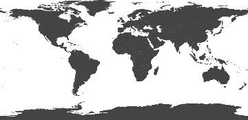
2D Earth
In[]:=
zem2D=Graphics[{Raster[ImageData[pic2],{{-6378,-6378},{6378,6378}}]}]
Out[]=
2D Earth + longitude + latitude
In[]:=
aa=Table[Line[{{-Pi,iPi/8},{Pi,iPi/8}}],{i,0,8,1}];bb=Table[Line[{{-Pi+iPi/8,0},{-Pi+iPi/8,Pi}}],{i,0,16,1}];zem2DRozvinuta=Graphics[{{Texture[pic1],Polygon[{{-Pi,0},{Pi,0},{Pi,Pi},{-Pi,Pi}},VertexTextureCoordinates{{0,0},{1,0},{1,1},{0,1}}]},aa,bb}]
Out[]=
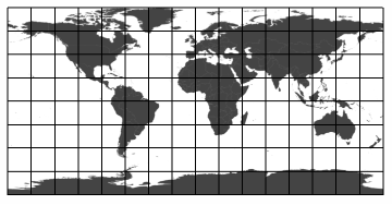
Elliptical trajectory
Elliptical trajectory
Equations
Equations
In[]:=
rElipsa[h_,μ_,e_,θ_]:=h^2/μ1/(1+eCos[θ])vElipsa[μ_,a_,r_]:=Sqrt[-μ/a+2μ/r]tElipsa[μ_,a_]:=2Pi/Sqrt[μ]a^(3/2)εElipsa[μ_,a_]:=-1/2μ/aeAnomaly[e_,θ_]:=2ArcTan[Sqrt[(1-e)/(1+e)]Tan[θ/2]]trueAnomaly[Ee_,e_]:=2ArcTan[Sqrt[(1+e)/(1-e)]Tan[Ee/2]]mAnomaly[Ee_,e_]:=Ee-eSin[Ee]time[Me_,μ_,e_,h_]:=h^3Me/(μ^2(1-e^2)^(3/2))
True anomaly when time is defined
True anomaly when time is defined
In[]:=
KeplerovProblemDefinedTime[μ_,n_,e_,h_,t_]:=Module[{Mt,riesenieEt,Et,θt,rt,xt,yt,zt},Mt=tn;riesenieEt=FindRoot[Mt==mAnomaly[Et,e],{Et,0}];Et=Et/.riesenieEt;θt=trueAnomaly[Et,e];rt=rElipsa[h,μ,e,θt];xt=rtCos[θt];yt=rtSin[θt];zt=0;Return[{t,Mt,Et,θt,rt,xt,yt,zt}]];KeplerovProblemForTimeInterval[μ_,n_,e_,h_,t_,timestep_]:=Module[{casoveBody},casoveBody=Table[KeplerovProblemDefinedTime[μ,n,e,h,ti],{ti,0,t,t/timestep}];Return[casoveBody]]
Time when true anomaly is defined
Time when true anomaly is defined
Two body problem 3D
Two body problem 3D
Analyze the 3D motion of the satellite in relative motion along an elliptical orbit around the Earth for an eccentricity value of 0.8. The distance from the Earth’s surface in periapsis is 1000 km. The position of the orbital plane is defined by Ω=45°, i=28°, the position of the elliptical orbit in the plane is defined by ω=30°. Ignore the mass of the satellite in the calculations. Consider the μEarth and rEarth parameters defined above.
Tasks:
1. trajectory in the plane of the orbit
2. trajectory in 3D space
Excercise 11:
3. Create the movement of the satellite in 3D space (timesteps = 3000, end time = 1 period)
4. Show satellite position on 2D map.
Tasks:
1. trajectory in the plane of the orbit
2. trajectory in 3D space
Excercise 11:
3. Create the movement of the satellite in 3D space (timesteps = 3000, end time = 1 period)
4. Show satellite position on 2D map.
Input parameters
Input parameters
1. trajectory in the plane of the orbit
1. trajectory in the plane of the orbit
angular momentum
r in periapsis
r in apoaspis
semi major axis
period
mean angular velocity
plot of 2D trajectory
Euler angles - transformation Perifocal (PQW) to Geographic coordinate system (IJK)
Euler angles - transformation Perifocal (PQW) to Geographic coordinate system (IJK)
transformation Perifocal CS - GCS
trajectory as a function of time
trajectory as a function of time
3. Create the movement of the satellite in 3D space (timesteps = 3000, end time = 1 period)
3. Create the movement of the satellite in 3D space (timesteps = 3000, end time = 1 period)
4. Show satellite position on 2D map.
4. Show satellite position on 2D map.
Assignment 2 (15 points)
Assignment 2 (15 points)
Process this assignment for trajectory of selected satellite.
Sum up key informations about the satellite and its trajectory.
TASK 1
Create 4 static points on the trajectory and connect them with line:
- periapsis & apsis, (2p)
- ascending node & descending node. (4p)
Create a dynamic/moving point on earth ground - intersection between satellite and center of earth. (3p)
Show this task in one Manipulate - orbit in 3D view.
TASK 2
Include the speed of the earth’s rotation to satellite position on 2D map. (4p)
Plot three periods. (2p)