A Single Pair Bell Correlation experiment, using a ‘pseudo’ unbunching transformation of polarization measurements. A updated single pair Bell Inequality type measurement done in Summer School 2023 has resulted in the proper Bell correlation result. Typical Bell experiments use four pairs of correlation measurements, and use BBO based non classical quantum entangled sources. This single angle pair Bell test simulation is based on using a bunched Poissonian beam, along with a ‘pseudo’ unbunching operator. This unbunching transformation is mathematical. Consequently, a direct single pair experiment would require a BB0 crystal based correlated beam. This single pair ‘pseudo unbunching translation operator’ has a surprising relationship with the quantum correlation equation.
Introduction
Introduction
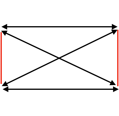
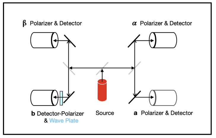
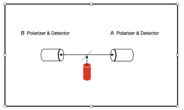
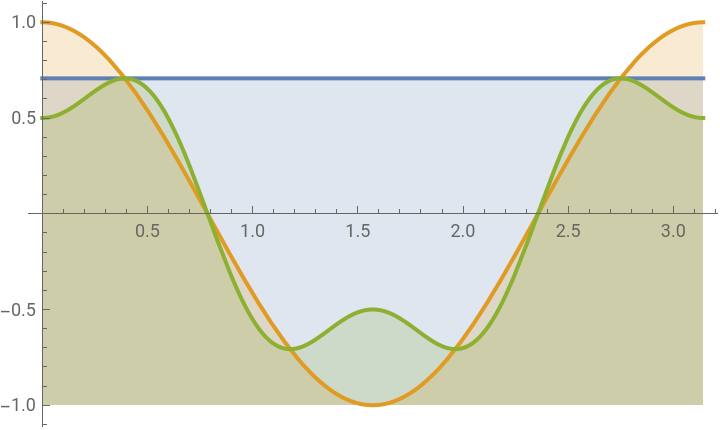
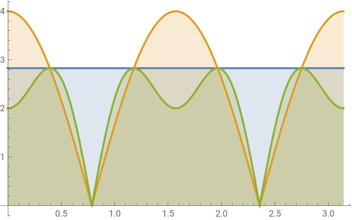
In Wolfram Summer School 23, a general form of the Aspect diagram was found for an arbitrary number of polarization pair measurements. Both the coincidence measurements, and the absolute value measurements are shown below for n = 1, 2, and 4 pairs. However, any number of pairs from 1 to n give the same forms for both the correlation, and absolute value measurements. The standard Bell test is for 4 pairs, where two pairs out of 6 are eliminated experimentally. This can be confirmed visually by looking at the red lines in the rectangle below.(For completeness, real coincidence data includes coincidences, singles, and nulls for each event pair. Here, we will look at the singles, and then the coincidences derived with the unbunching transformation.)
In[]:=
TablePlot,n(Cos[2k]),
n
2
n
4
(3Cos[2k]-Cos[3(2k)])
,{k,0,π},Filling->Bottom,{n,{1,2,4}}Out[]=
,
,
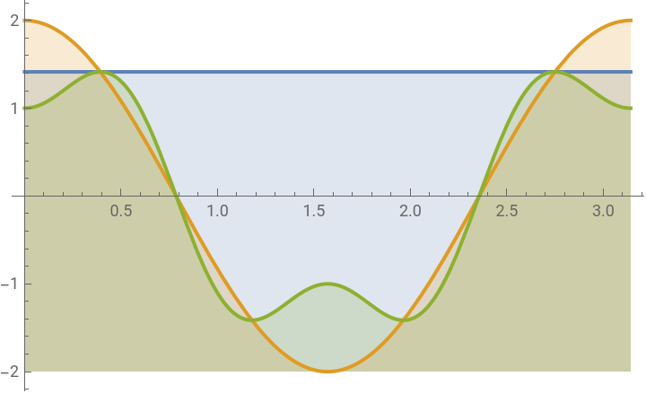
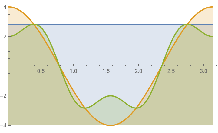
TablePlot,Abs[n(Cos[2k])],,π,Filling->Bottom,{n,{1,2,4}}
n
2
Abs(3Cos[(2k)]-Cos[3(2k)])
n
4
,k,-0.01π
8
Out[]=
,
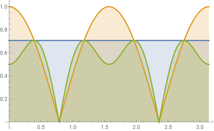
,
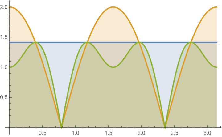
The experimental setup starts with a polarized 2mw 633nm Thor solid state laser, with linear polarizers in front of all beams. A beam splitter splits the output into two beams. One polarizer is fixed at 90 degrees in front of one of the beams. The 2nd beam’s polarization is measured in 5 degree increments for a total of 180 degrees (π ), and stored in the dataD31 file. A subset of dataD31 is used here, as well as dataD32 dataD33, and dataD34, in order to contain error-bar information. The polarization measurements in dataD31 are all positive or zero for all angles because they are not coincidence measurements.
For an initial sub-study, we shall measure the n = 1 polarizer pair case, for 7 single polarization angles with denominators of 60 and 20:
For an initial sub-study, we shall measure the n = 1 polarizer pair case, for 7 single polarization angles with denominators of 60 and 20:
In[]:=
Forn=0,n<7,n++,Print,30(0+n)
(1+10n)π
60
,0,,30,,60,,90,,120,,150,,180
π
60
11π
60
7π
20
31π
60
41π
60
17π
20
61π
60
The results for the 7 polarization measurements
are all non-negative, and are plotted below on the red curve. The desired coincidence curve is green. Our first goal is to understand the relationship between the red curve and the green curve, in order to derive a transformation to turn the red curve into the green curve. This will correspond to a ‘pseudo’ unbunching curve which turns a polarization measurement into a correlation measurement. The desired green curve
below is the QM correlation curve
given by Cos2k-
π
25
π
60
shift in the measurement axis
is due to the polarizer slipping 3 degrees as it is tightened during installation in our case.The Bell inequality pre-absolute value case is initially suppressed below with a 0
4
ShowPlot-1,,1+Cos2k-3Cos2k-Cos32k,k,,π+,Filling->Bottom,ListPlot[dataD31],Ticks->,,,,,,,-1,0,,,1,1.5
1
2
Cos2k-
,π
25
1
2
π
25
,
-
1
2
1-Cos2k-
π
25
,
0
4
-
π
25
-
π
25
-π
64
π
61
π
60
11π
60
7π
20
31π
60
41π
60
17π
20
61π
60
1
2
1
2
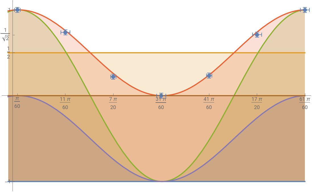
Looking at the graph above, it is possible to see that the red curve minus the parallel purple curve results in the green correlation curve:
In[]:=
1
2
π
25
-
1
2
1
-
Cos2k-
π
25
Out[]=
1
2
π
25
1
2
π
25
Expanding the above, we can see that the resulting green curve, is the quantum mechanical correlation equation:
In[]:=
1
2
1
2
π
25
1
2
1
2
2
k
-
π
25
Cos2k-
π
25
It is remarkable that the green transformation, which contains
Cos[2k -
π
25
]
quantum correlation curve, that is the goal of our ‘measurement based’ simulation, can be derived from the -
1
2
1
-
Cos2k-
π
25
Cos[2k -
π
25
]
itself, and which is directly related to our measurement data, in such a simple and direct manner.This is verified by putting our 7 measurements into dataD31, using the 7 point subset below:dataD31=
Around,0.03,Around,0.03
π
60
152.65
152.65
,
Around,0.05,Around,0.03
11π
60
112.45
152.65
,
Around,0.03,Around,0.03
7π
20
33.7
152.65
,
Around,0.05,Around,0.03
31π
60
0
152.4
,
Around,0.03,Around,0.03
41π
60
35.625
152.65
,
Around,0.05,Around,0.03
17π
20
108.35
152.65
,
Around,0.05,Around,0.03
61π
60
152.4
152.65
{{0.052±0.030,1.000±0.030},{0.58±0.05,0.737±0.030},{1.100±0.030,0.221±0.030},{1.62±0.05,0.000±0.030},{2.147±0.030,0.233±0.030},{2.67±0.05,0.710±0.030},{3.19±0.05,0.998±0.030}}
We now verify that the measurement points lie on the shift, and in multiples of π as follows:
green correlation curve
. The correlation equivalent purple measurement operator
shift for each measurement point is calculated below. We calculate the corresponding 7 offset angles: { 0, 30, 60, 90
,120,150, 180 in degrees} with the appropriate π
25
Including these offset shift values above, along with the error bars results in dataD32, as calculated below. The blue numerators of the second terms in each of the 7 points below correspond to the shifted values above. The error bars with 0.05 instead of 0.03 are because 5 degree increment ticks are very difficult to see. (Perhaps this problem can be avoided in the future using motor controlled polarizers as well as data loggers.)
The offsets for each angle are:
The offsets for each angle are:
Including these offset values along with the error bars results in dataD32
gives the results in dataD33 below.
Here too, the error bars with 0.05 instead of 0.03 are because 5 degree increment ticks
are very difficult to see.
(Perhaps this problem can be avoided in the future using motor controlled polarizers,
and data loggers.)
The content of dataD33 with error bars is calculated below is shown as light green:
Below, the Bell curves are superimposed on top of the measurement and simulation, showing that the quantum mechanics curve fits the data, not the Bell curves. Here, we add the Bell curves for comparison by turning on the brown equation below.
The below code is the ‘absolute value transformation’ for the 3 negative measurement points; this is done by changing the negative values to positive values as is done with the Abs function :
This is the measurement using 36 data points. Using this curve would also produce the same results as transformed plot 3 above.
A Conclusion, a Status Update and a Perspective
A Conclusion, a Status Update and a Perspective
From the above perspective, only the first, yet important step has been taken.
Next steps include:
Next steps include:
◼
Investigating the real unbunched single pair, single photon version of the Bell experiment, with a type 1 BBO crystal.
◼
Directly doing single and multiple pair Bell experiments with unbunched type 2 BBO crystal sources.
◼
Creating and measuring invisible Wolfram Multiway diagrams using a type 1 and 2 BBO crystal sources.
◼
Creating and measuring Wolfram Multiway diagrams using visible modern entangled sources, possibly in 2nd and higher orders.
◼
Output of Multiway diagrams corresponding to specific angles, as well as as entanglements of entanglements.
◼
Learning and expanding the new quantum framework in Mathematica for the above efforts.
◼
More work is required to link the new quantum framework to QuantumToMutiway.
Other associated works have included and shall further include:
◼
Examples of beam characterization based on spec sheets from a dot laser vendor
◼
Characterizing light in terms Poissonian, as well as
◼
Second order g(2) measurements, and other non-classical quantum optical activities.
References
References
Quantum Optics, an introduction by Mark Fox.
Acknowledgements
Acknowledgements
My deepest appreciations to:
◼
Steven Wolfram
◼
Xerxes Arsiwalla
◼
Hatem Elshatlawy
◼
Nick Murzin
◼
Shivam Sawarn, and
◼
All the numerous Wolfram Summer and Winter School support people.
They are the ones who make all this possible.
CITE THIS NOTEBOOK
CITE THIS NOTEBOOK
A Single Pair Bell Correlation measurement, using a 'pseudo' unbunching operator
by Mark Merner
Wolfram Community, STAFF PICKS, January 11, 2024
https://community.wolfram.com/groups/-/m/t/3100273
by Mark Merner
Wolfram Community, STAFF PICKS, January 11, 2024
https://community.wolfram.com/groups/-/m/t/3100273