ORIGINAL ARTICLE: Federico Bertacco, Ewain Gwynne, Scott Sheffield (2023), Scaling limits of planar maps under the Smith embedding. arXiv:2306.02988v1.
DOI: https://doi.org/10.48550/arXiv.2306.02988
GITHUB: https://github.com/federico-bertacco/smith-embedding
DOI: https://doi.org/10.48550/arXiv.2306.02988
GITHUB: https://github.com/federico-bertacco/smith-embedding
Article Abstract: The Smith embedding of a finite planar map with two marked vertices, possibly with conductances on the edges, is a way of representing the map as a tiling of a finite cylinder by rectangles. In this embedding, each edge of the planar map corresponds to a rectangle, and each vertex corresponds to a horizontal segment. Given a sequence of finite planar maps embedded in an infinite cylinder, such that the random walk on both the map and its planar dual converges to Brownian motion modulo time change, we prove that the a priori embedding is close to an affine transformation of the Smith embedding at large scales. By applying this result, we prove that the Smith embeddings of mated-CRT maps with the sphere topology converge to -Liouville quantum gravity (-LQG).
γ
γ
The code below generates a random walk in conditioned to end where it started after steps. The code starts by computing , which is the 45-degree-rotated version of whose coordinates are independent one-dimensional walks conditioned to end at zero. It then displays two figures, one showing the trace of the walk in and the other plotting the and coordinates separately as functions of time.
(X,Y)
2
n
(A,B)
(X,Y)
2
X
Y
n=5000;Z=Table[0,{j,1,n+1}];A=Z;B=Z;For[j=1,j<n,++j,A[[j+1]]=A[[j]]+If[2RandomReal[]>1+A[[j]]/(n-j),1,-1];B[[j+1]]=B[[j]]+If[2RandomReal[]>1+B[[j]]/(n-j),1,-1]];X=n/2+(A+B)/2;Y=n/2+(A-B)/2;Row[{ListPlot[{X,n+Sqrt[n]-Y},Joined->True,Axes->False,ImageSize->315],Graphics[Table[Line[{{X[[j]],Y[[j]]},{X[[j+1]],Y[[j+1]]}}],{j,1,n}],ImageSize->315]}]
Out[]=
The graph of determines a tree obtained by identifying points connected by a chord under the graph, with the two endpoints of identified so that chords can wrap around. An embedding of such a tree is shown below in blue (with a similar tree for shown in green).
X
[0,n]
Y
In[]:=
vertnumX=Z+1;vertnumY=Z+1;last=Z+1;minxloc=1;minyloc=1;For[j=1,j<n+1,++j,If[X[[j]]<X[[minxloc]],minxloc=j];If[Y[[j]]<Y[[minyloc]],minyloc=j]];count=1;For[j=minxloc,j<n+1,++j,If[X[[j+1]]>X[[j]],vertnumX[[j+1]]=++count;last[[X[[j+1]]]]=count,vertnumX[[j+1]]=last[[X[[j+1]]]]]];vertnumX[[1]]=vertnumX[[n+1]];For[j=1,j<minxloc-1,++j,If[X[[j+1]]>X[[j]],vertnumX[[j+1]]=++count;last[[X[[j+1]]]]=count,vertnumX[[j+1]]=last[[X[[j+1]]]]]];vertnumY[[minyloc]]=++count;last=Z+count;For[j=minyloc,j<n+1,++j,If[Y[[j+1]]>Y[[j]],vertnumY[[j+1]]=++count;last[[Y[[j+1]]]]=count,vertnumY[[j+1]]=last[[Y[[j+1]]]]]];vertnumY[[1]]=vertnumY[[n+1]];For[j=1,j<minyloc-1,++j,If[Y[[j+1]]>Y[[j]],vertnumY[[j+1]]=++count;last[[Y[[j+1]]]]=count,vertnumY[[j+1]]=last[[Y[[j+1]]]]]];Row[{GraphPlot[SimpleGraph[Table[Style[vertnumX[[j]]<->vertnumX[[j+1]],Blue],{j,1,n}]],VertexStyle->Blue,GraphLayout->{"SpringEmbedding"},ImageSize->315],GraphPlot[SimpleGraph[Table[Style[vertnumY[[j]]<->vertnumY[[j+1]],Green],{j,1,n}]],VertexStyle->Green,GraphLayout->{"SpringEmbedding"},ImageSize->315]}]
Out[]=
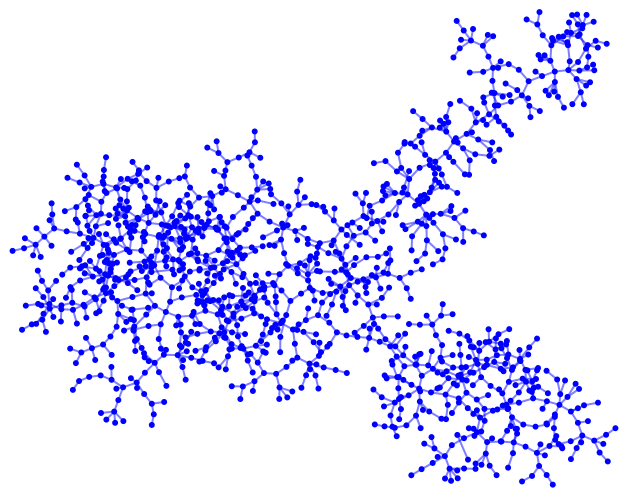
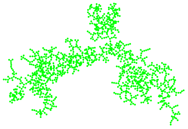
We can then draw in the red edges between the blue and green trees to construct and illustrate a graph object as follows.
In[]:=
g=Table[0->0,{j,1,3n/2}];count=1;For[j=1,j<=n,++j,g[[count++]]=Style[vertnumX[[j]]<->vertnumY[[j]],Red]];For[j=1,j<=n,++j,If[X[[j]]<X[[j+1]],g[[count++]]=Style[vertnumX[[j]]<->vertnumX[[j+1]],Blue]]];For[j=1,j<=n,++j,If[Y[[j]]<Y[[j+1]],g[[count++]]=Style[vertnumY[[j]]<->vertnumY[[j+1]],Green]]];GraphPlot3D[g,VertexStyle->Table[i->If[i<vertnumY[[minyloc]],Blue,Green],{i,1,n/2+2}],GraphLayout->{"SpringElectricalEmbedding"}]
Out[]=

Alternatively, one can represent the graph using a sparse array , which is more efficient when the number of vertices is large. The code below displays only the red edges, so the map is a quadrangulation.
M
In[]:=
M=SparseArray[Table[0,{j,1,n/2+2},{k,1,n/2+2}]];For[j=1,j<n+1,j++,M[[vertnumX[[j]],vertnumY[[j]]]]+=1];x=GraphPlot3D[M,GraphLayout->{"SpringElectricalEmbedding"},VertexShapeFunction->None]
Out[]=

Replacing the square-embedding function sq with a cylinder-embedding function rsvq gives an embedding in the cylinder. Here we only display squares of size about some cutoff so that computational time is not wasted on drawing squares that may be too small to see.
A similar function spsq (using a Mercator projection) gives an embedding in the sphere instead of cylinder.
We remark that one can also type the following after any of the 3D figures to export an animation showing a rotating version of the image.
CITE THIS NOTEBOOK
CITE THIS NOTEBOOK
Scaling limits of planar maps under the smith embedding
by Federico Bertacco
Wolfram Community, STAFF PICKS, June 16, 2023
https://community.wolfram.com/groups/-/m/t/2939113
by Federico Bertacco
Wolfram Community, STAFF PICKS, June 16, 2023
https://community.wolfram.com/groups/-/m/t/2939113