In this project we explore 1+1D Euclidean Dynamical Triangulations using standard Metropolis Algorithm.
1+1D Euclidean Dynamical Triangulations
1+1D Euclidean Dynamical Triangulations
Any quantum field theory can be described by Path Integrals where all possible trajectories contribute to the transition amplitude. A common way to define and regularize the functional integral is to discretize the space-time coordinates and approximate each path by linear pieces. In general Relativity gravity is encoded in the space-time geometry. Here, the geometry of four-dimensional space-time plays the role of the trajectory. All space-time histories contribute to the transition amplitude. Euclidean Dynamical Triangulations (EDT) is such an approach where the functional integral is discretized the 2D space-time surface via triangles.
Implementation
Implementation
In 1+1D EDT, one-dimensional state with a topology S1 is built from links with length 'a' and 2D space-time surface are built from equilateral triangles with the curvature is localized at vertices. The aim is to calculate the amplitude of a transition between two geometric states.
Each geometry is obtained by gluing together triangles. To compute the path integral, the space of all geometries is explored by a random walk with the starting point a minimal sphere, the triangulation with the topology of a sphere in 2-dimensions. To achieve this, the standard function in Mathematica to discretize a region with a mesh is used.
Each geometry is obtained by gluing together triangles. To compute the path integral, the space of all geometries is explored by a random walk with the starting point a minimal sphere, the triangulation with the topology of a sphere in 2-dimensions. To achieve this, the standard function in Mathematica to discretize a region with a mesh is used.
The starting point:
In[]:=
Needs["NDSolve`FEM`"]ClearAll[init2Dtriangulation,discreteCylinder];(*Inializethetriangulationin2Dwhichisaculinderwithagivenradiusandheight*)init2Dtriangulation[r_,h_,len_]:=Module[ {ℛ,disCyl}, ℛ=ImplicitRegion[-r≤x≤r&&-h/2≤z≤h/2&&-r≤y≤r&&(x^2+y^2==r^2),{x,y,z}]; disCyl=DiscretizeRegion[ℛ,MaxCellMeasure{"Length"len}]]discreteCylinder=init2Dtriangulation[0.1,0.1,4]
Out[]=
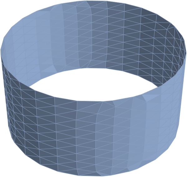
The mesh is then converted to a graph using the adjacency matrix
The mesh is then converted to a graph using the adjacency matrix
In[]:=
ClearAll[getAdjacencyMatrix];(*Gettheadjacencymatrixfromamesh-allthenodeswhichareconnected*)getAdjacencyMatrix[R_]:=Module[{linesIn},linesIn=MeshCells[R,1][[All,1]];Normal[SparseArray[Table[{linesIn[[i,1]],linesIn[[i,2]]}1,{i,1,Dimensions[linesIn][[1]]}]]]](*demo*)getAdjacencyMatrix[discreteCylinder]ClearAll[getGraphFromMesh];(*Getthegraphfrommeshusingtheadjacencymatrix*)getGraphFromMesh[dis_]:=AdjacencyGraph[getAdjacencyMatrix[dis],VertexCoordinatesMeshCoordinates[dis],DirectedEdgesFalse](*demo*)triCylGraph=getGraphFromMesh[discreteCylinder]
Out[]=
Out[]=
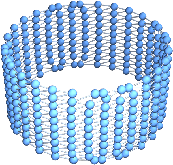
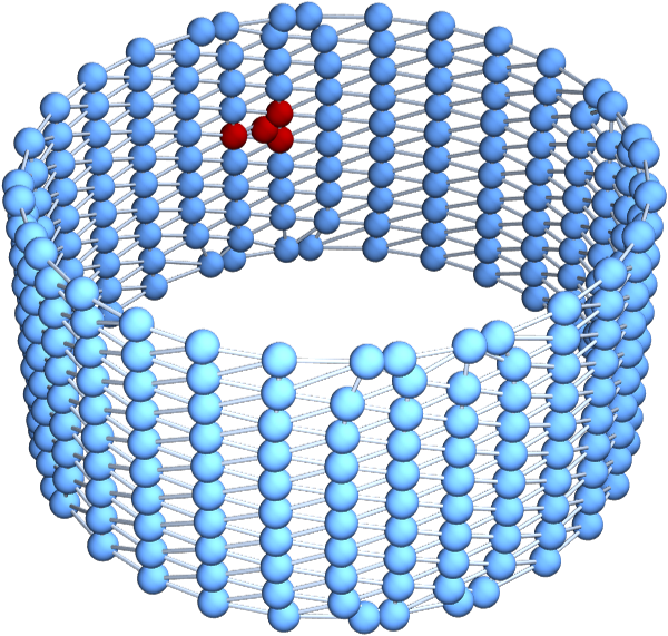
The new geometry in the random walk must remain valid triangulations, must maintain the same topology as the original configuration and the process of generating new geometries must be ergodic. In 2 dimensions, the three moves are inserting a node, deleting a node and flipping a link.
In[]:=
ClearAll[insertNode,smallestMissing];smallestMissing[list_]:=With[{n=SelectFirst[Ordering[list],#≠list[[#]]&]},If[n===Missing["NotFound"],Length@list+1,n]];Options[insertNode]={"HighlightStep"False};insertNode[graph_,OptionsPattern[]]:=Module {vertices=Sort@VertexList[graph],v1,nbhd1,v2,nbhd2,v3Candidates,v3,newv,newvCoords}, (*Print["I"];*) v1=RandomChoice[vertices]; nbhd1=AdjacencyList[graph,v1]; v2=RandomChoice[nbhd1]; nbhd2=DeleteCases[AdjacencyList[graph,v2],v1]; v3Candidates=Intersection[nbhd1,nbhd2]; If Length@v3Candidates>0, v3=RandomChoice[Intersection[nbhd1,nbhd2]]; newv=smallestMissing[vertices]; newvCoords=Total[GraphEmbedding[graph][[{v1,v2,v3}]]]3; If[ OptionValue["HighlightStep"], HighlightGraph[Graph[EdgeAdd[VertexAdd[graph,newv],{v1newv,v2newv,v3newv}],VertexCoordinates{v1GraphEmbedding[graph][[v1]],v2GraphEmbedding[graph][[v2]],v3GraphEmbedding[graph][[v3]],newvnewvCoords}],{v1,v2,v3,newv}(*,GraphHighlightStyle"VertexDiamond"*)], Graph[EdgeAdd[VertexAdd[graph,newv],{v1newv,v2newv,v3newv}],VertexCoordinates{v1GraphEmbedding[graph][[v1]],v2GraphEmbedding[graph][[v2]],v3GraphEmbedding[graph][[v3]],newvnewvCoords}] ], graph ;Graph[insertNode[triCylGraph,"HighlightStep"True]]
Out[]=
Concluding remarks
Concluding remarks
Euclidean Dynamical Triangulations were successfully implemented in 1+1D and the evolution was studied in Monte Carlo time. Future work involves the study of the Euclidean Dynamical Triangulations within the Wolfram Model.
Keywords
Keywords
◼
Wolfram Summer School
◼
Wolfram Physics Project
◼
Euclidean Dynamical Triangulations
Acknowledgment
Acknowledgment
This project was completed under the guidance of my mentor Jack Heimrath. The project was defined by Stephen Wolfram, so the author acknowledges him, along with Jonathan Gorard for the valuable discussions and insights.
References
References
◼
J. Laiho, S. Bassler, D. Coumbe, D. Du, and J. T. Neelakanta. Lattice
Quantum Gravity and Asymptotic Safety. 2016.
Quantum Gravity and Asymptotic Safety. 2016.
◼
J. Ambjorn, J. Jurkiewicz, and R. Loll. Recent results in Euclidean dynamical triangulations. arXiv:1701.06829.
◼
Scott David Bassler. Euclidean Dynamical Triangulations: Running Couplings and Curvature Correlation Functions. https://surface.syr.edu/cgi/viewcontent.cgi?article=2105&context=etd