In this post, we show how the Tectonic puzzle (also known as Jigsaw Sudoku or Suguru) can be solved using graph coloring algorithms. By viewing the puzzle grid as a graph that represents adjacency rules, block constraints and given hints, we can apply standard graph-theory coloring methods to find valid solutions. This perspective illustrates how many logic puzzles can be naturally understood through graph theory and how the same approach can be extended to similar puzzles.
Introduction
Introduction
Building on the post “How to Solve Sudoku Using Graph Theory” (also available as a video on the Wolfram R&D YouTube channel), we extend the approach of using graph-coloring techniques to find valid solutions to the Tectonic puzzle (also known as Jigsaw Sudoku or Suguru). As we will see, solving a Tectonic puzzle using graph theory closely follows the process used for standard Sudoku, with the main difference lying in the structure of the corresponding graph.
In Tectonic, the blocks are irregularly shaped, arranged like a jigsaw or tectonic plates. Blocks can consist of one, two, three, four, or five cells, and the goal is to place the numbers 1 through 5 in each block, depending on its size. For example, a block with one cell can only contain the number 1, while a block with two cells must contain both 1 and 2, and so on. One key constraint is that cells containing the same number may never touch each other, neither horizontally, vertically, or diagonally.
Out[]=
1 | 1 | |||||||
2 | 3 | |||||||
4 | 4 | 4 | ||||||
1 | ||||||||
4 | 5 | 4 | 5 | |||||
3 | ||||||||
2 | 5 |
I have to be honest: having extra hints and fewer numbers to fill in makes me think that Tectonic puzzles are easier to solve than standard Sudoku puzzles. Many people who are new to Tectonic would disagree and consider it trickier than normal Sudoku, mainly because the irregular shapes disrupt familiar visual patterns. However, once you let go of this visual restriction, the puzzle can often be solved efficiently, especially when using tools such as pencil marking to keep track of the irregular hints and possible values. The need for pencil marking arises because Tectonic’s irregular structure increases the complexity of tracking possibilities and constraints. Paradoxically, this same irregularity is precisely what makes graph-coloring algorithms a natural and powerful framework for finding solutions to Tectonic puzzles.
Tectonic
Tectonic
As mentioned earlier, in a Tectonic puzzle the blocks can consist of one, two, three, four, or five cells, and the numbers 1 through 5 must be placed within them. A block with one cell can only contain the number 1, while a block with two cells must contain both 1 and 2, and so on. An important constraint is that cells containing the same number may never touch each other, not horizontally, vertically, or diagonally.
As can be seen, the irregular blocks do not need to be square and have no regular pattern. This irregularity is one of the main challenges of the puzzle, as it makes creating and displaying the grid more complicated. For example, even displaying the blocks requires a custom function to render the puzzle correctly:
Tecton[tectons_,givens_:0]:=Module,;
In addition to the custom display function, extra information is required to specify which cells belong to each block:
In[]:=
tectons={{{1,1},{1,2},{2,1},{2,2},{3,1}},{{1,3},{1,4},{1,5},{2,3},{2,4}},{{1,6},{1,7},{2,5},{2,6},{3,5}},{{1,8},{2,7},{2,8},{3,6},{3,7}},{{1,9},{2,9},{3,9},{4,8},{4,9}},{{3,8}},{{5,8}},{{5,9},{6,8},{6,9},{7,8},{7,9}},{{4,6},{4,7},{5,6},{5,7},{6,7}},{{5,5},{6,5},{6,6},{7,4},{7,5}},{{5,2},{5,3},{6,3},{6,4},{7,3}},{{3,3},{3,4},{4,4},{4,5},{5,4}},{{3,2},{4,1},{4,2},{4,3},{5,1}},{{6,1},{6,2},{7,1},{7,2}},{{7,6},{7,7}}};
In[]:=
Tecton[tectons]
Out[]=
Additional information is also needed to define the location of each given hint:
In[]:=
givens=<|{1,1}->1,{2,2}->2,{3,1}->4,{1,4}->1,{2,8}->3,{3,3}->4,{3,9}->4,{4,4}->1,{5,1}->4,{5,3}->5,{5,5}->4,{5,7}->5,{6,8}->3,{7,5}->2,{7,9}->5|>;
In[]:=
Tecton[tectons,givens]
Out[]=
1 | 1 | |||||||
2 | 3 | |||||||
4 | 4 | 4 | ||||||
1 | ||||||||
4 | 5 | 4 | 5 | |||||
3 | ||||||||
2 | 5 |
To find a solution for a Tectonic puzzle, many of the same standard techniques used in Sudoku can be applied. One simple approach involves eliminating possible values by checking whether a number already appears in the same block or in neighboring cells. By repeatedly applying these basic elimination rules, players can gradually fill in more digits.
Other solution methods are also possible, for example, in a post by Sander on Solving Suguru (Tectonic) puzzles, a systematic candidate-elimination algorithm is described. This approach iteratively applies elimination rules in a loop until no further progress can be made. (Actually, the puzzle setup used here is adapted from Sander’s work, from which the puzzle definition, including the blocks and given hints, is taken).
However, as puzzles become more challenging, these basic techniques may no longer be sufficient. In particularly difficult cases, more advanced methods such as depth-first recursive backtracking are required, as noted in Sander’s work. To avoid this added complexity and to develop a more general solution method, we instead turn to graph coloring, which provides a systematic and powerful framework for solving Tectonic puzzles.
Graph Coloring
Graph Coloring
A graph consist of a set of vertices (also called nodes) and a set of edges that connect pairs of vertices. Let’s consider an example graph with the set of vertices {1, 2, 3, 4} and the set of edges {12, 13, 14, 24, 34}.
Out[]=
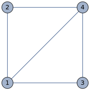
Graph coloring involves assigning different colors to the vertices of a graph in such a way that no two adjacent vertices share the same color. An important step of this is to determine the minimum number of colors required to color the graph’s vertices, which is known as the Chromatic Number. For this example the Chromatic Number is 3:
In[]:=
VertexChromaticNumber[g]
Out[]=
3
Intuition Behind Graph Coloring
Intuition Behind Graph Coloring
To understand the intuition behind graph coloring, let’s consider a simplified example. We have a graph and our goal is to assign colors to the nodes in such a way that no two adjacent nodes share the same color.
As previously seen, for this graph we have a Chromatic Number of 3, meaning we need three colors, for which we will take Blue, Red, and Green. To assign colors to the vertices of the graph, we can employ a recursive function that traverses the graph and assigns colors to the nodes.
Let’s start with Node 1. We select a color from the color list, let’s take our first color: Blue, and attempt to assign it to Node 1. However, before assigning the color, we need to check if any of the adjacent nodes (nodes connected to Node 1) already have the same color.
Out[]=
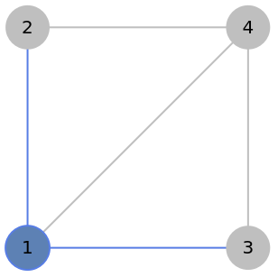
If any adjacent node has the same color we cannot assign the color to the node because it would violate the rule of no two adjacent nodes having the same color. In such cases, we need to select a different color from the available color list and repeat the process.
In this example, none of the adjacent nodes to Node 1 have the color Blue, so we can assign Blue to Node 1.
Out[]=
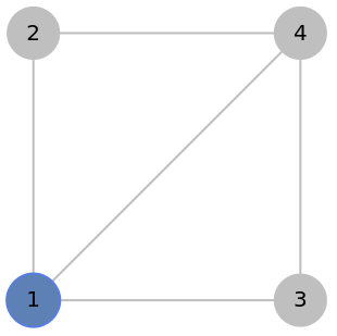
We have colored Node 1 with the color Blue. Now we need to move on to the next node, we will move to Node 2. To color Node 2, we select a color from the color list, once again let’s take our first color: Blue.
Out[]=
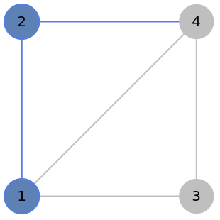
However, since Node 2 is adjacent to Node 1, which already has the color Blue, we cannot assign Blue to Node 2. We need to explore alternative colors from the color list, and in this case, the next color is Red.
Out[]=
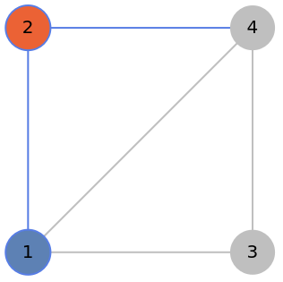
None of the adjacent nodes have the color Red, so we can assign Red to Node 2.
Now we have colored Node 1 and Node 2 with the colors Blue and Red, respectively. We need to move on to the next node: Node 3. To color Node 3, we select a color from the available color list, once again let's start with Blue.
Out[]=
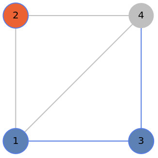
However, Node 3 is adjacent to Node 1, which already has the color Blue. Therefore, we can not color Node 3 with Blue. We need to try the next color, which is Red.
Out[]=
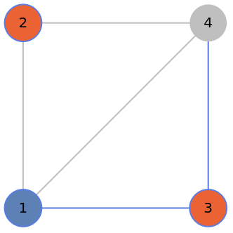
None of the adjacent nodes have the color Red, so we can assign Red to Node 3.
Although Node 3 can also be colored with the next color in the list: Green, we are trying to minimize the number of colors used, so this is not a good option.
Continuing with Node 4, we select a color from the available color list, once again let’s start with Blue.
Out[]=
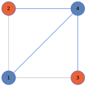
Since Node 1 is already colored with Blue, we cannot assign Blue to Node 4 as it is adjacent to Node 1. Hence, we proceed to the next available color, which is Red.
Since Node 2 and 3 are already colored with Red, we cannot assign Red to Node 4 as it is adjacent to Node 2 and 3. Hence, we proceed to the next available color, which is Green.
Now we check all the adjacent nodes again to verify if any of them are already colored with Green, this is not the case, so we can color Node 4 with Green.
In this case, we can see that the entire graph can be colored with 3 colors: Blue, Red, and Green. Thus, the chromatic number of this graph is indeed 3.
As we saw the recursive function traverse the graph, selecting a color for every vertex and checking its compatibility with the adjacent nodes at each step. If a color is found that satisfies the adjacency constraint for a particular node, it is assigned to that node. And this process continues until all nodes in the graph are assigned colors.
Luckily, Wolfram Language (WL) already has a function that finds the optimal vertex coloring. This function can be used to automate the process of assigning colors to the vertices of a graph, ensuring that no two adjacent nodes share the same color in the following way:
How Sudoku can be solved using Graph Coloring
How Sudoku can be solved using Graph Coloring
Now that we understand the idea behind vertex coloring: assigning a color to each vertex of a graph so that no two adjacent vertices share the same color; we can see how this is essentially the same as finding the number that goes in each cell of a puzzle on the tectonic puzzle. With this connection in mind, we can now apply graph-coloring techniques to solve a Tectonic puzzle.
As an example, we will consider the following Tectonic puzzle:
As an example, we will consider the following Tectonic puzzle:
Tectonic graph
Tectonic graph
The first step in using graph coloring to find a solution is to represent the puzzle grid as a graph. In this representation, the Tectonic graph consists of n vertices, where each vertex corresponds to a single cell in the Tectonic grid.
Once the vertices are defined, the next step is to establish the connections between them. To do this, we assign a unique tag to each vertex corresponding to its location in the Tectonic grid. This allows us to determine which vertices should be connected based on their relative positions (row, column, and block) and puzzle constraints.
Once we have the unique tag for each vertex , we connect each node to its row and column neighbors, that is, to the cells directly above, below, to the left, and to the right. This step creates the basic grid structure of the graph:
For example, if we consider vertex 39, we can see that it is connected to its immediate row and column neighbors:
These connections allow vertices to interact and exchange information during the solving process. However, this is not yet sufficient, since Tectonic puzzles also forbid equal numbers in diagonally adjacent cells. To incorporate this constraint, we add connections between diagonal neighbors. This ensures that vertices sharing a diagonal edge are also treated as adjacent in the graph:
For example, if we consider vertex 39, we can see that it is connected to its immediate diagonal neighbors:
By combining the horizontal, vertical, and diagonal connections, we obtain a graph that fully represents the adjacency constraints of the puzzle grid:
For example, if we consider vertex 39, we can see that it is connected to all its immediate neighbors:
The final structural component comes from the Tectonic blocks themselves. Cells belonging to the same block must all contain different numbers, so we represent this constraint by connecting every pair of vertices within the same block. In graph terms, each block is modeled as a complete graph:
By establishing these connections, we obtain a fully connected graph that captures all the rules of the Tectonic puzzle:
If we again highlight vertex 39, we now see connections not only to it’s grid and diagonal neighbors, but also to all other vertices within its block:
It is important to note that while the grid and diagonal connections remain the same across puzzles of the same size, the block-based connections depend on the specific layout of each Tectonic puzzle and will therefore vary from puzzle to puzzle.
Tectonic Problem
Tectonic Problem
We now integrate the given hints, or preset numbers, into the graph. To do this, we begin by identifying the positions of all given numbers, the 1s, 2s, 3s, 4s, and 5s, and group them accordingly. We also include singleton blocks, where only the number 1 is allowed by definition.
To illustrate this process, we focus first on the number 2. To incorporate the hints into the graph, we connect each vertex labeled with a given 2 to all other vertices that contain given numbers different from 2. These connections enforce that such vertices must have different colors, which adds useful constraints and helps the graph-coloring algorithm converge more efficiently:
We apply the same procedure to every other vertex labeled with the number 2, connecting it to all given vertices that are not 2:
When all these edges are combined, we obtain the complete structure representing the constraints associated with the number 2:
This structure ensures that all vertices corresponding to the number 2 share the same color and have a different color from all vertices that do not correspond to the number 2. This process is repeated for each given number in the puzzle. As a result, the graph becomes more interconnected and accurately captures the relationships imposed by the given hints:
Finally, we address an additional constraint related to block size. In Tectonic, if a block contains fewer than five cells, for example, a block of size 3, only the numbers 1 through 3 are allowed. To enforce this in the graph, we connect every vertex in such a block to all given hints with values greater than the block size. For instance, if a block of size 4 appears in the lower-left corner of the grid, we connect its vertices to all vertices representing the number 5, this ensures that the color corresponding to 5 cannot be assigned within that block:
And the connections for this block will look like this:
We repeat this process for every block of size n, connecting it to all given hints with value n + 1 and higher. And the full strucutre will look like this:
Graph coloring
Graph coloring
In the context of a Tectonic puzzle, this corresponds to assigning numbers to cells while respecting block sizes and ensuring that the same number does not appear in neighboring cells, horizontally, vertically, or diagonally. This formulation aligns directly with the concept of the chromatic number in graph theory, since we can construct the graph by connecting vertices that must be assigned different colors. Since the numbers 1 through 5 can be represented as colors, five distinct colors are required to solve the puzzle. This corresponds directly to the concept of the chromatic number in graph theory:
We therefore only need to construct the full Tectonic graph, incorporating grid adjacency, diagonal constraints, block constraints, and the given hints:
Once the graph is built, we can visualize the resulting coloring:
The final step is simply to translate each color back into its corresponding number.
When this translation is applied across the grid, we obtain the complete solution to the Tectonic puzzle:
Therefore, to solve the puzzle, we only need to specify the block structure and the given hints:
Find an appropriate graph coloring:
And then, translate the coloring into the corresponding numbers:
It is important to note that this approach works for any valid Tectonic puzzle, regardless of the number of solutions. Even if a puzzle has multiple valid solutions, or infinitely many, the graph-coloring algorithm will still find a correct solution that satisfies all constraints, ensuring that no adjacent cells share the same color.
To demonstrate the flexibility of this method, we can apply it to a larger puzzle as well. For example, consider a 12×10 Tectonic puzzle:
This puzzle cannot be solved using simple elimination or brute-force methods. To solve it using graph coloring, we construct the graph, find a valid coloring and translate the coloring into the solution:
We can then observe the final solution:
Conclusion
Conclusion
We have examined how graph theory and graph coloring techniques can be adapted to solve Tectonic Sudoku puzzles. By representing the Tectonic Sudoku grid as a graph, where cells are vertices and edges connect cells that share a region or meet specific puzzle constraints we can apply graph coloring algorithms to assign numbers to the cells while respecting the puzzle’s unique rules. This approach allows for a structured and systematic method to find valid solutions. Tectonic Sudoku introduces additional constraints compared to standard Sudoku, making graph-based approaches particularly useful for managing these complex relationships.
Beyond Tectonic Sudoku, graph theory and coloring techniques have broad applications in combinatorial optimization and problem solving, providing powerful tools for addressing not only puzzles but also a wide range of real-world problems that can be modeled as graph-based challenges.
References
References
◼
Solving Suguru (tectonic) puzzles by Sander Huisman, Wolfram Community, STAFF PICKS, 2016 https://community.wolfram.com/groups/-/m/t/2983903
◼
Solving Sudoku puzzles with Graph Theory by Alejandra Ortiz Duran, Wolfram Community, STAFF PICKS, 2023 https://community.wolfram.com/groups/-/m/t/2983903
CITE THIS NOTEBOOK
CITE THIS NOTEBOOK
How to solve tectonic puzzles using graph theory
by Alejandra Ortiz Duran
Wolfram Community, STAFF PICKS, January 21, 2026
https://community.wolfram.com/groups/-/m/t/3614977
by Alejandra Ortiz Duran
Wolfram Community, STAFF PICKS, January 21, 2026
https://community.wolfram.com/groups/-/m/t/3614977