Control of a Stirred-Tank Heating Process
Authors: Housam Binous and Ahmed Bellagi
Control of a Stirred-Tank Heating Process
Authors: Housam Binous and Ahmed Bellagi
Authors: Housam Binous and Ahmed Bellagi
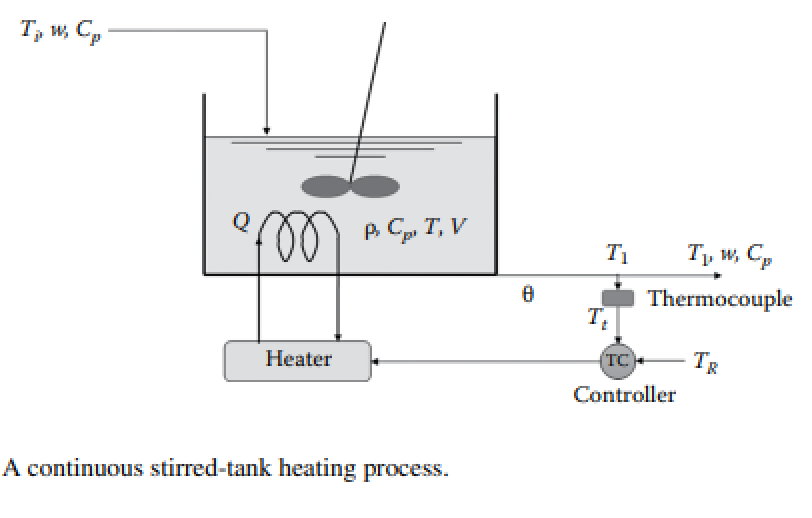
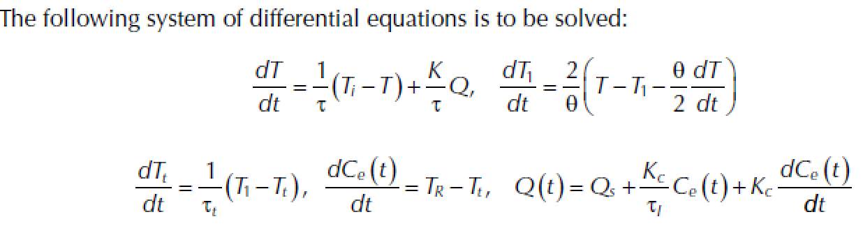
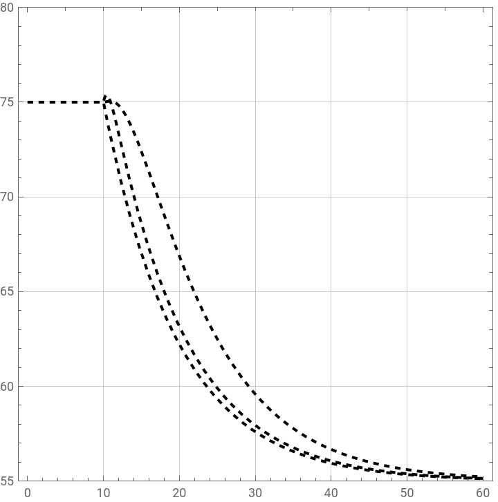
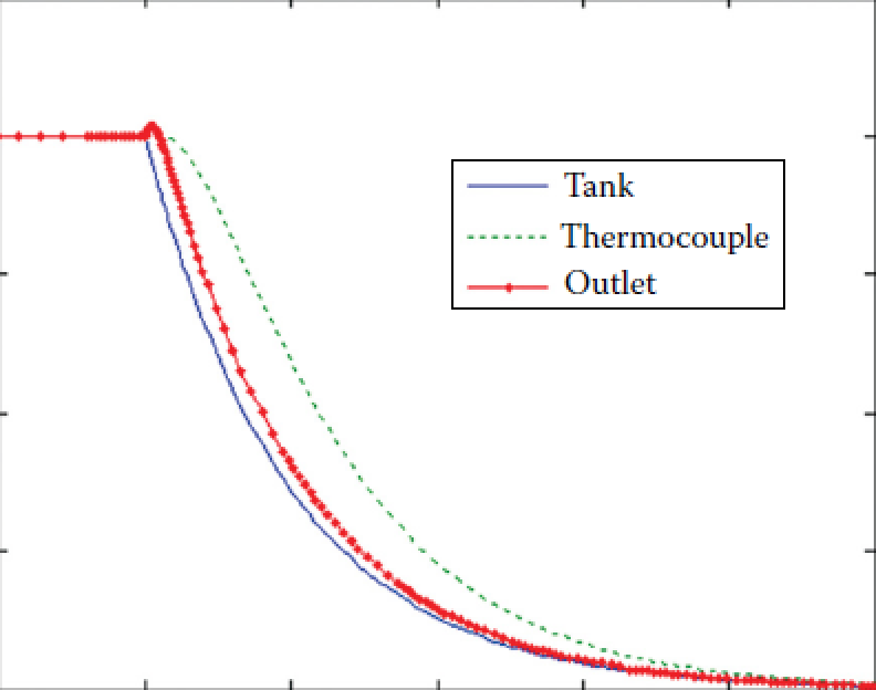
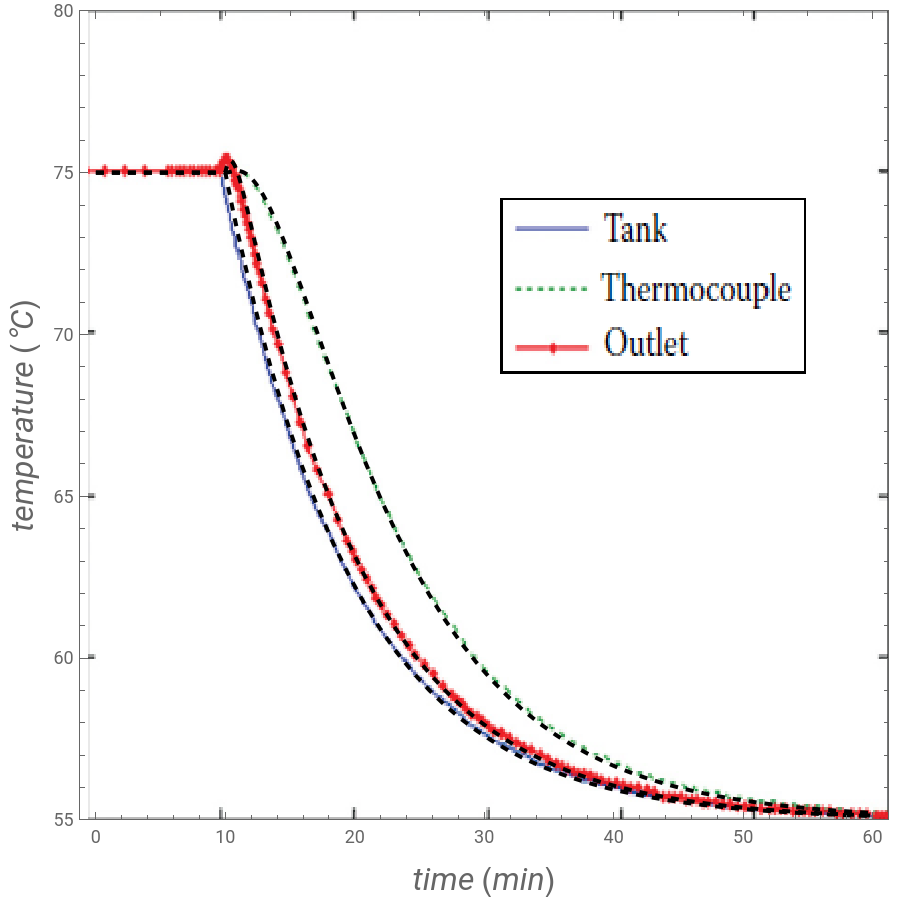
Figure below shows a continuous stirred-tank heating process.This process consists of a stirred tank, heater, and PI controller. The liquid is fed at a constant mass flow rate of w = 250 kg/min and temperature Ti = 50°C. Liquid properties are the following: the density is equal to ρ = 980 kg/m3 and the heat capacity is taken equal to Cp = 1.6 kJ/(kg · °C). The tank’s volume is equal to V = 2.5 m3. A set-point temperature TR = 75°C is selected. The outlet temperature is measured by a thermocouple as Tt. The heat flux Q (kJ/min) supplied by the heater is manipulated by either a P only or a PI controller with Kc = 60 kJ/(min· °C) and τI = 1.8 min. The thermocouple exhibits 1st-order dynamics with time constant τt = 3 min and unity gain. The time delay between the heating tank and the thermocouple is θ = 1.2 min.The following scenarios are selected:1. The system is initially operating at steady state at a temperature of 75°C (set-point). The inlet temperature Ti is suddenly changed to 30°C at time t = 10 min. Assuming no control actions (open-loop, Kc = 0), we plot the profiles of the fluid temperature in the tank T, the measured temperature Tt, and the fluid outlet temperature T1.2. If the controller is engaged (closed loop), we plot the profiles of T, Tt, and T1.3. If the PI controller is replaced by a proportional (P) controller with Kc = 60 kJ/(min· °C), we plot the profiles of T, Tt, and T1.For each scenario, our results, obtained by either NDSolve or InverseLaplaceTransfom, are superimposed to their counterparts given in Example 9.18 of Ref. 1.References:[1] Yeo, Yeong Koo, Chemical engineering computation with MATLAB, Boca Raton : Taylor & Francis, CRC Press, 2017.

Open loop response or no control action
In[]:=
rho=980;V=2.5;Cp=1.6;w=250;taut=3.6;theta=1.2;TR=75;tauI=1.8;K=1/(Cp*w);tau=rho*V/w;
In[]:=
Ti[t_]:=If[t<10,50,30]
In[]:=
Qs=(TR-50)/K
Out[]=
10000.
In[]:=
Kc=0;
In[]:=
Q[t_]:=Qs+(Kc/tauI)*IntErr[t]+Kc*(TR-Tt[t]);sys={T'[t](Ti[t]-T[t])/tau+K*Q[t]/tau,T1'[t]2*(T[t]-T1[t]-(theta/2)*T'[t])/theta,Tt'[t](T1[t]-Tt[t])/taut};
In[]:=
init={T[0]75,T1[0]75,Tt[0]75};
In[]:=
sol=NDSolve[Join[sys,init],{T,T1,Tt},{t,0,60},AccuracyGoal10]
Out[]=
TInterpolatingFunction,T1InterpolatingFunction,TtInterpolatingFunction


In[]:=
p1=Plot[{T[t]/.sol,T1[t]/.sol,Tt[t]/.sol},{t,0,60},PlotRange{55,80},PlotRangeAll,FrameTrue,AspectRatio1,GridLinesAutomatic,PlotStyle{{Dashed,Thick,Black},{Dashed,Thick,Black},{Dashed,Thick,Black}}]
Out[]=
In[]:=
IMG=
;
In[]:=
Show[p1,ImageSize450{1,1},Prolog{Raster[ImageData[IMG,DataReversedTrue],{Scaled[{0.01,0.0}],Scaled[{1,1.00}]}]},FrameLabel{Style["time (min)",16,Italic],Style["temperature (°C)",16,Italic]}]
Out[]=
Closed loop response - proportional only control action
In[]:=
Kc=60;
In[]:=
Q[t_]:=Qs+Kc*(TR-Tt[t]);
In[]:=
sys={T'[t](Ti[t]-T[t])/tau+K*Q[t]/tau,T1'[t]2*(T[t]-T1[t]-(theta/2)*T'[t])/theta,Tt'[t](T1[t]-Tt[t])/taut};
Closed loop response - proportional-integral control action