Let me review the muddled notion of “spacefilling curve”. Around 1900, Giuseppe Peano and David Hilbert shocked everybody by discovering continuous maps of (one dimensional) intervals onto solid patches of 2-space. These were “curves” only in the strict sense. They were anything but smooth, and their graphs were blobs instead of arcs. In order to define them, Peano and Hilbert sketched recursive line drawings. Unfortunately, math popularizers confused these sketches with the actual spacefilling functions, and the term “spacefilling curve” has come to mean one of these recursive diagrams, with no understanding of how, or even if, they actually fill space. https://en.wikipedia.org/wiki/Dragon_curve is a typical example of this sad state of affairs. The curves they are talking about are merely polygonal approximations to graphs of the wonderful dragon function, which they never mention. If they did, it would be a lame function merely from dyadic rationals to dyadic rationals.
Julian Ziegler Hunts wrote the following function to evaluate fractal curves at rational points and similarly recursively-defined functions. Usually dragon curves, Hilbert curves, etc. and their inverses.
In[]:=
piecewiserecursivefractal[x_,f_,which_,iters_,fns_]:=piecewiserecursivefractal[x,g_,which,iters,fns]=((piecewiserecursivefractal[x,h_,which,iters,fns]:=Block[{y},y/.Solve[f[y]==h[y],y]]);Union@@((fns[[#]]/@piecewiserecursivefractal[iters[[#]][x],Composition[f,fns[[#]]],which,iters,fns])&/@which[x]))
Given the recursive, schematic description of a fractal, it creates an exact mathematical function, or even its multivaled inverse! Thus the Dragon Function, whose graphs include the so-called Dragon Curve, has the definition
In[]:=
dragun[t_]:=piecewiserecursivefractal[t,Identity,Piecewise[{{{1},0<=#<=1/2},{{2},1/2<=#<=1}},{}]&,{2*#&,2*(1-#)&},{(1+I)*#/2&,(I-1)*#/2+1&}]
This is a new way to program! Whereas the traditional, schematically defined Dragon is defined only on dyadic rationals:
In[]:=
dragun/@Range[0,1,1/8](*andproducesonlyGaussiandyadicrationals,*)
Out[]=
{0},-+,,+,+,+,,-,{1}
1
4
4
2
1
4
4
1
2
2
3
4
4
1
2
3
4
4
we can now evaluate it for any rational:
In[]:=
dragun/@Range[0,1,1/7]
Out[]=
{0},-+,+,+,+,+,-,{1}
1
5
2
5
1
5
3
5
2
5
5
4
5
2
5
2
5
5
3
5
5
Notice that dragun[3/7] = dragun[5/7] = 2/5 + i/5, the lower endpoint of the common boundary where two dragons join to form the next larger one:
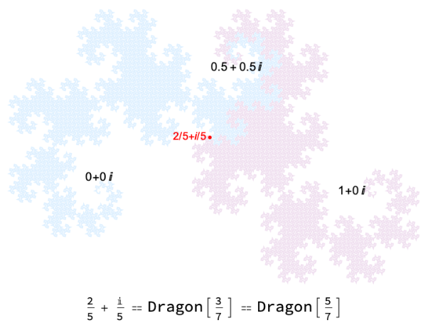
How silly to study a function when you can express neither the abscissa nor the ordinate of such an important point! And when you can’t express inverses at all! But with piecewiserecursivefractal, we can even handle a few irrationals!
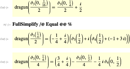
Here is the inverse Dragon function:
In[]:=
undrag[z_]:=piecewiserecursivefractal[z,Identity,If[-1/3<=Re[#]<=7/6&&-1/3<=Im[#]<=2/3,{1,2},{}]&,{#*(1-I)&,(1-#)*(1+I)&},{#/2&,1-#/2&}]
In[]:=
undrag[2/5+I/5]
Out[]=
,
3
7
5
7
Take a look near 2/5 + i/5. Imagine writing a function that merely says True or False whether its argument is in that Dragon image.
In[]:=
undrag[1/6+I/3]
Out[]=
,,
13
60
7
20
23
60
A triple point.
In[]:=
dragun/@%
Out[]=
+,+,+
1
6
3
1
6
3
1
6
3
The longest closed loop in the Dragon function is the image of that closed interval [3/7, 5/7]:
In[]:=
tim[xp_]:=(Print[#[[1]],",",Length[#[[2]]]];#[[2]])&@AbsoluteTiming[xp](*tim is my identity function that interjects elapsed time and length.*)SetAttributes[tim,HoldAll];
In[]:=
Graphics[{Line[{ReIm@First@dragun@#&/@Range[0/7,3/7,1/7/512],ReIm@First@dragun@#&/@Range[5/7,7/7,1/7/512]}],Red,Line[ReIm@First@dragun@#&/@Range[3/7,1/2,1/7/512/2]],Blue,Line[ReIm@First@dragun@#&/@Range[1/2,5/7,1/7/512/2]]}]//tim
69.1198,1
Out[]=
(red ⋃ blue). It can be arbitrarily lengthened by revisiting double and triple points once or twice. A Dragon fed a dithered ramp
In[]:=
Table[(m+1/2+(-1)^m/4)/64,{m,0,63}]
Out[]=
,,,,,,,,,,,,,,,,,,,,,,,,,,,,,,,,,,,,,,,,,,,,,,,,,,,,,,,,,,,,,,,
3
256
5
256
11
256
13
256
19
256
21
256
27
256
29
256
35
256
37
256
43
256
45
256
51
256
53
256
59
256
61
256
67
256
69
256
75
256
77
256
83
256
85
256
91
256
93
256
99
256
101
256
107
256
109
256
115
256
117
256
123
256
125
256
131
256
133
256
139
256
141
256
147
256
149
256
155
256
157
256
163
256
165
256
171
256
173
256
179
256
181
256
187
256
189
256
195
256
197
256
203
256
205
256
211
256
213
256
219
256
221
256
227
256
229
256
235
256
237
256
243
256
245
256
251
256
253
256
ListLinePlot[ReIm[dragun[#][[1]]]&/@%,AspectRatio->Automatic](*appearstoself-avoid:*)
Out[]=
But in fact, all spacefilling functions are dense with triple points! The usual Hilbert Curve:
In[]:=
hilbert[t_]:=piecewiserecursivefractal[t,Identity,{Min[4,1+Floor[4*#]]}&,{1-4*#&,4*#-1&,4*#-2&,4-4*#&},{I*(1-#)/2&,(I+#)/2&,(I+1+#)/2&,1+#*I/2&}]
In[]:=
ListLinePlot[ReIm[First[hilbert@#]]&/@Range[1/6/64,1,1/64],AspectRatio->Automatic]
Out[]=
Both Numberphile and 3Blue 1Brown perpetrate this atrocity. Two other sampling frequencies, replacing Line by Polygon:
One of Hilbert’s ancient ancestors.
Expositors of spacefilling shun the vanilla Heighway Dragon because it self contacts in a grid, completely disguising where it’s going. Mandelbrot’s solution was the “median curve”, which averages pairs of consecutive points. But this almost seems like a different curve. Not! Julian realized that the “median” of two draguns is exactly one dragun on a dithered ramp:
Replacing Line with Polygon in the Graphics:
Smoothing twice more, we get the Penguin Curve!
But is there a sampling frequency that self-avoids without dithering? Sort of!
Huh? You call that self-avoidance? Watch if we replace Line with Polygon!
Here is frame 118 (~ 355/3) of a “beat frequency” (phase drift) of a twindragon,
showing the traditional square grid at the east and west ends, drifting to the “4094 self-avoidance” at NE and SW. Of course I must nag that “self-avoiding spacefiller” is a monstrous oxymoron. Spacefillers self-contact like crazy. Every simply connected area contains an infinitude of triple points.