COVID19: Italian SIRD estimates and prediction
COVID19: Italian SIRD estimates and prediction
Christos Papahristodoulou
May 24, 2020
May 24, 2020
In this document I apply the standard SIRD model , using Italian COVID19 data. Up to date, May 23, there are 89 daily observations, starting from February 24. The model is adjusted and does not cover all possible people to be infected, but only those who been tested and were found positive until May 23. In Italy more than 3.3 million tests were curried so far and the accumulated number of infected people is 228,658 (almost 7%). The infected/tested ratio over the recent days is very low, at most 1% (about 650 new infected per day), compared to more than 30% two months ago. Today is the 89th day and I will solve the problem to predict the key variables until the middle of June (t = 115). Assuming the current number of new infected is around 600 per day, the susceptible population is therefore set equal to about 245,000 over the period under investigation.
After I have retrieved the data, I use 79 out of 89 observations to estimate the key SIRD parameters. Thereafter, using these estimates I solve the system of ODE equations and plot their paths together with the current observations.
Retrieving the data
In[]:=
URLDownload["https://raw.githubusercontent.com/pcm-dpc/COVID-19/master/dati-andamento-nazionale/dpc-covid19-ita-andamento-nazionale.csv",Directory[]<>"\\pd.read_csv(url)"];
In[]:=
SemanticImport["https://raw.githubusercontent.com/pcm-dpc/COVID-19/master/dati-andamento-nazionale/dpc-covid19-ita-andamento-nazionale.csv"];
Since I will apply the standard SIRD model, I will use the following columns (all are accumulated statistics): infected (7), recovery (10), deaths (11), and total (12).
Estimates on parameters
In order to estimate the key SIRD (Susceptible, Infected, Recovery, Death) parameters, β, γ, δ, I will use 79/89 of the observations (until May 13).
In[]:=
infstart=Import["https://raw.githubusercontent.com/pcm-dpc/COVID-19/master/dati-andamento-nazionale/dpc-covid19-ita-andamento-nazionale.csv",{"Data",2;;80,7}];recstart=Import["https://raw.githubusercontent.com/pcm-dpc/COVID-19/master/dati-andamento-nazionale/dpc-covid19-ita-andamento-nazionale.csv",{"Data",2;;80,10}];deathstart=Import["https://raw.githubusercontent.com/pcm-dpc/COVID-19/master/dati-andamento-nazionale/dpc-covid19-ita-andamento-nazionale.csv",{"Data",2;;80,11}];totstart=Import["https://raw.githubusercontent.com/pcm-dpc/COVID-19/master/dati-andamento-nazionale/dpc-covid19-ita-andamento-nazionale.csv",{"Data",2;;80,12}]//Reverse;
I need to normalize the data by dividing their values by 221,216, i.e. the total infected number until May 13. The model is:
eqS=s'[t]-βs[t]m[t];eqI=m'[t]βs[t]m[t]-γm[t]-δm[t];eqR=r'[t]γm[t];eqD=q'[t]δm[t];
where, s = susceptible, m = infected, r = recovery, q = deaths.
In[]:=
time=Range[79];
In[]:=
datastart=Thread[Join[{time},{totstart}/221216,{infstart}/221216,{recstart}/221216,{deathstart}/221216]]//N;
In[]:=
f[β_?NumericQ,γ_?NumericQ,δ_?NumericQ]:=Sum[Total[(yi[[i,All]]-Map[pfun[β,γ,δ][[i]],xi])^2],{i,1,4}]//Quiet
data=datastart;(*takeonly79days*)xi=data[[1,All]];(*independentvariable*)yi=data[[2;;5,All]];(*fourdependentvariables*)pfun=ParametricNDSolveValue[{s'[t]-βs[t]m[t],m'[t]βs[t]m[t]-γm[t]-δm[t],r'[t]γm[t],q'[t]δm[t],s[xi[[1]]]yi[[1,1]],m[xi[[1]]]yi[[2,1]],r[xi[[1]]]yi[[3,1]],q[xi[[1]]]yi[[4,1]]},{s,m,r,q},{t,0,80},{β,γ,δ}];(*thetimeperiodissetto80days*)
In[]:=
fit=NMinimize[f[β,γ,δ],{β,γ,δ}];params=fit//Last
Out[]=
{β0.200637,γ0.0222591,δ0.00896591}
Solve the SIRD system using the estimated parameters
Using these estimates I solve the system of ODE equations and plot their paths together with the current observations.
In[]:=
Clear[t];
In[]:=
Clear[s,m,r,q];
In[]:=
Clear[β,γ,δ];
In[]:=
eqS=s'[t]-βs[t]m[t];eqI=m'[t]βs[t]m[t]-γm[t]-δm[t];eqR=r'[t]γm[t];eqD=q'[t]δm[t];
In[]:=
β=0.200637;γ=0.0222591;δ=0.00896591;
In[]:=
solu=NDSolve[{eqS,eqI,eqR,eqD,s[0]1,m[0]0.00096,r[0]0,q[0]0},{s,r,m,q},{t,115}];(*initiallytherewereabout220persons*)
In[]:=
soluS=First[s/.solu];soluI=First[m/.solu];soluR=First[r/.solu];soluD=First[q/.solu];
In[]:=
Plot[{soluS[t],soluI[t],soluR[t],soluD[t]},{t,0,115},PlotRange{0,1},PlotStyle{Blue,Red,Green,Magenta},PlotLegends{"Susceptible","Infected","Recovered","Dead"}]
Out[]=


Plot the data and the solution of the ODE
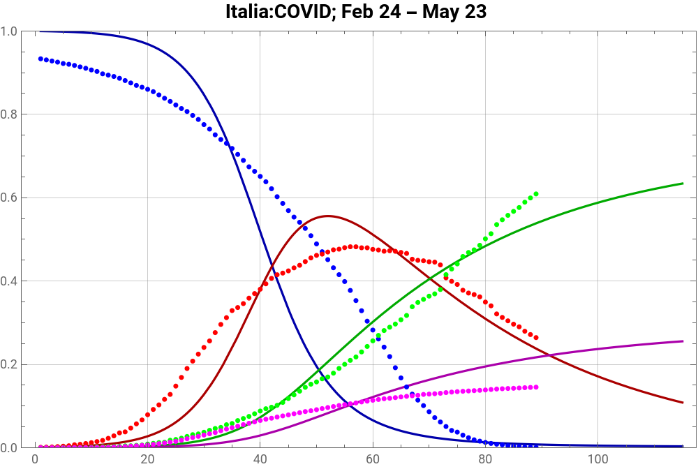
We can now plot all data as well as the ODE.
In[]:=
infall=Import["https://raw.githubusercontent.com/pcm-dpc/COVID-19/master/dati-andamento-nazionale/dpc-covid19-ita-andamento-nazionale.csv",{"Data",2;;90,7}];recall=Import["https://raw.githubusercontent.com/pcm-dpc/COVID-19/master/dati-andamento-nazionale/dpc-covid19-ita-andamento-nazionale.csv",{"Data",2;;90,10}];deathall=Import["https://raw.githubusercontent.com/pcm-dpc/COVID-19/master/dati-andamento-nazionale/dpc-covid19-ita-andamento-nazionale.csv",{"Data",2;;90,11}];totall=Import["https://raw.githubusercontent.com/pcm-dpc/COVID-19/master/dati-andamento-nazionale/dpc-covid19-ita-andamento-nazionale.csv",{"Data",2;;90,12}]//Reverse;
We normalize again these data by dividing their values by 245,000, i.e. the total expected number of infected, by the middle of June.
In[]:=
beta=ListPlot[Tooltip[{totall/245000,infall/224500,recall/224500,deathall/224500}],PlotStyle{Blue,Red,Green,Magenta},PlotLegends{"Susc","Inf","Rec","Dead"}];
In[]:=
Show[Plot[{soluS[t],soluI[t],soluR[t],soluD[t]},{t,1,115},PlotLabelStyle["Italia:COVID; Feb 24 - May 23 ",Black,Bold,14],PlotRange{0,1},PlotStyle{Darker[Blue],Darker[Red],Darker[Green],Darker[Magenta]},GridLinesAutomatic,FrameTrue,PlotRangeAll,ImageSize500],beta]
Out[]=


In[]:=
Manipulate[Show[Plot[a{soluS[t],soluI[t],soluR[t],soluD[t]},{t,1,T},PlotRangeAutomatic],beta,PlotStyle{Darker[Blue],Darker[Red],Darker[Green],Darker[Magenta]},ImageSize450,EvaluatedTrue,PlotPoints1000,GridLinesAutomatic,FrameTrue,PlotTheme"Detailed"],{{T,90},50,115,Appearance"Labeled"},{{a,0.94},0.9,1.0,Appearance"Labeled"},ControlPlacementTop,AlignmentRight,SaveDefinitionsTrue]
Out[]=


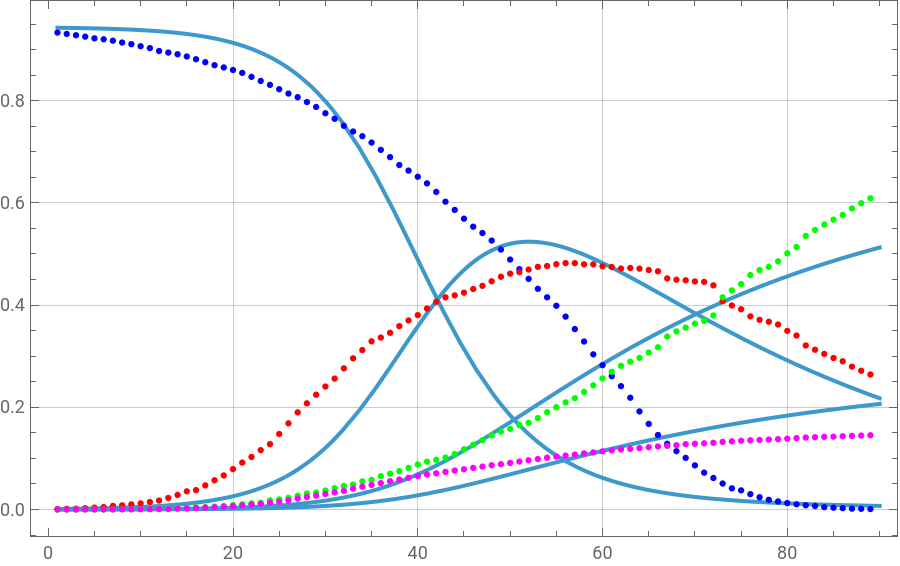


Today, on May 23, the model overestimates the number of deaths by 49,526 - 32,616 = 16,976 , underestimates the number of infected by 59,322 - 54,380 = 4,941 and the number of recovery by 136,720 - 123,120 = 13,600. Notice also that the theoretical value of Susceptible should be 754 less, there will be 24,778 still infected and the number of deaths will increase to slightly above 58,000 by the middle of June. Regarding the “low” number of deaths compared to the theoretical higher value, there is a lot of discussion in Italy if all COVID19 deaths outside the hospitals have been reported correctly. Some media argue that the true value should be at least 19,000 higher. In that case our predictions are rather close to these estimates. Finally, the actual Ro value is 0.07, while its start value was around 9.