This notebook series is designed to introduce selected dynamic economic models to both advanced undergraduate and graduate students. Economists have relied on a series of economic models to better understand the otherwise highly complex causal relationship among many economic variables. Dynamic economic models set up by systems of either difference or differential equations are particularly useful in tracing the change in the quantity of unknown economic variables (e.g., the capital stock, demand for labor, aggregate output, etc.) and their interactions over time.
This notebook series aims to help students better understand the depth, usefulness, and limitations of major existing micro and macroeconomic models by demonstrating how we can use Wolfram Mathematica to replicate and reconstruct the core ideas and find dynamic solution of the model.
The model introduced in this notebook series include, among others, (1) the cobweb model of the quantity and price adjustment, (2) Keynes’s aggregate demand model, (3) Hicks’s ISLM model, (4) Samuelson’s investment accelerator model, (5) Kalecki’s investment delay model, (6) the predator-prey interaction model, (7) the epidemic model, (8) Ricardo’s three dimensional business cycle model, (9) Marx-Goodwin business cycle and growth model, (10) Smith’s and Ricardo’s growth model, (11) the Harrod-Domar growth model, (12) the Solow growth model, (13) the RBC model, (14) Romer’s new growth model, and (15) the circuit of capital model.
The predator-prey system
Introduction
Introduction
The predator-prey system is one of the most important mathematical models initially designed by mathematical biologists. The model is based upon a system of nonlinear differential equations that describes the population growth of two species that are interacting with one another. The model captures dynamic interactions between two species, one of which plays a role as a predator in the sense that it requires other species for its own sustenance and biological reproduction. How the population of these two species changes, while exhibiting their predator-prey interactions over time, is the key feature that we can observe by solving this system of differential equations (Note 1)
Note 1: A brief introduction to the history of this predator - prey model can be found at “Lotka-Volterra Equation” (https://en.wikipedia.org/wiki/Lotka%E2%80%93Volterra_equations) . There are a number of useful textbooks that introduce this model . This notebook is based upon a survey of Blanchard et al (2012), Hoy et al (2011), and Abell and Braselton (2016).
Since its inception, this model has been widely used to analyze various biological systems not only as a theoretical framework but also as a guide for empirical estimations and policies. Some economists and social scientists have also adopted this model to analyze various complex social and economic phenomena. As we will see later, David Ricardo’s business cycle theory can be reconstructed by a modified predatory-prey model. Richard Goodwin’s growth cycle is also fundamentally based upon the predator-prey interaction between wage share and employment rate of labor.
This note aims to provide a concise reference for this predator-prey model. For this purpose, this notebook offers a practical guide for building and solving the baseline predator-prey model and visualizing interactive solution curves as some crucial parameters change.
The predator-prey system with the exponential growth of the prey population
The predator-prey system with the exponential growth of the prey population
A general model
A general model
The model
The model
The classic example of the predator-prey model can be written as:
x |
y |
where α, β, γ, and δ are all positive growth parameters and both x > 0 and y > 0 are stock variables for two interacting species.
As the first differential equation =x(α-βy) indicates, the population of the species x grows exponentially with α being a fixed growth-rate-coefficient. But the population of the same species x decreases as it interacts with other species y by a factor of β xy. On the other hand, the population of the species y decreases exponentially (the parameter -γ represents this exponential decrease) in the absence of its interactions with other species x. The species y can only survive and reproduce its own species by interacting with its prey population x. How much and how fast the species y reproduces its own species and grows its population depends on the size of the positive growth parameter δ.
x
The steady state values and the local stability
The steady state values and the local stability
We can approach this system of two first-order nonlinear differential equations in several ways. First, let us find the steady state value by setting the two differential terms equal to zero. The steady state value is the hypothetical solution of the system when we assume that there is no more force of change. We can find this value by setting all the differential terms equal to zero and simplify the remaining terms further.
In[]:=
ClearAll[α,β,γ,δ,x,y];Solve[{x*(α-βy)0,y*(-γ+δx)0},{x,y}]
Out[]=
x,y,{x0,y0}
γ
δ
α
β
Notice that there are two steady state points, one of which is an attractor (or the “sink”) and the other being repelling point (or the “source”). One way of determining the (local) stability of the system behavior, we can evaluate Jacobian matrix at each steady state point. The Jacobian matrix is nothing more than the partial derivative of the system of two differential equations compiled in a compact matrix array. Depending on the sign of trace, determinant, and eigenvalue of this Jacobian matrix evaluated at each steady state value, we may have the system constantly moving away from the steady state value, converging toward this steady state value, and constantly oscillating around this steady state value (Hoy et. al 2012 provides an excellent summary).
In[]:=
J=
D[x*(α-βy),x] | D[x*(α-βy),y] |
D[y*(-γ+δx),x] | D[y*(-γ+δx),y] |
Out[]=
{{α-yβ,-xβ},{yδ,-γ+xδ}}
Now let us evaluate the value of this matrix near the two steady state values we identified earlier. For the steady state value (x, y) = (0, 0), the sign of trace is not determinable yet, while the sign of the determinant is negative, and the two eigenvalues are real in the same sign. Therefore, the steady state value (0, 0) is a source or repelling point.
In[]:=
Tr[J]/.{x0,y0}
Out[]=
α-γ
In[]:=
Det[J]/.{x0,y0}
Out[]=
-αγ
In[]:=
Eigenvalues[J]/.{x0,y0}//Simplify
Out[]=
α-γ-,α-γ+
1
2
2
(α+γ)
1
2
2
(α+γ)
For the steady state value, (x, y) = (,, the trace of the Jacobian matrix is zero, the determinant is positive, and the real part of two eigenvalues are opposite signs. Therefore, the solution curve must oscillate around this particular steady state value.
γ
δ
α
β
In[]:=
Tr[J]/.x,y
γ
δ
α
β
Out[]=
0
In[]:=
Det[J]/.x,y
γ
δ
α
β
Out[]=
αγ
In[]:=
Eigenvalues[J]/.x,y
γ
δ
α
β
Out[]=
-
-αγ
,-αγ
The static visualization of solution curves with fixed parameters
The static visualization of solution curves with fixed parameters
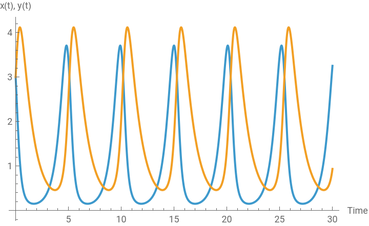
Next, let us assign some arbitrary values to undefined parameters and find the general solution numerically. Assuming that α = 2, β = 1.2, γ = 1, and δ = 0.9 and the initial condition of both species are x(0) = 3, y(0) = 3, let us compute the general numerical solution and determine the property of this system. For this purpose, we use a built-in function in Wolfram Mathematica, NDSolve [ ].
In[]:=
ClearAll[α,β,γ,δ,x,y,t];α=2;β=1.2;γ=1;δ=0.9;sol=NDSolve[{x'[t]==x[t]*(α-β*y[t]),y'[t]y[t]*(-γ+δ*x[t]),x[0]3,y[0]3},{x[t],y[t]},{t,30}]
Out[]=
x[t]InterpolatingFunction[t],y[t]InterpolatingFunction[t]


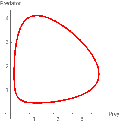
The NDSolve function generates two “InterpolatingFunctions” for each variable, which contain the trajectory (solution curve) of two variables. We can visualize this trajectory by using both Plot and ParametricPlot. The Plot function shows the value of each variable over time (the horizontal axis is “Time”, while the vertical axis is the value of x and y at time t), while the ParametricPlot shows the time-dependent interaction between the two variables.
In[]:=
Plot[Evaluate[{x[t],y[t]}/.sol],{t,0,30},PlotLegends{"prey","predator"},AxesLabel{"Time","x(t), y(t)"}]
Out[]=


In[]:=
ParametricPlot[Evaluate[{x[t],y[t]}/.sol],{t,0,30},PlotStyle{Red,Thick},AxesLabel{"Prey","Predator"}]
Out[]=
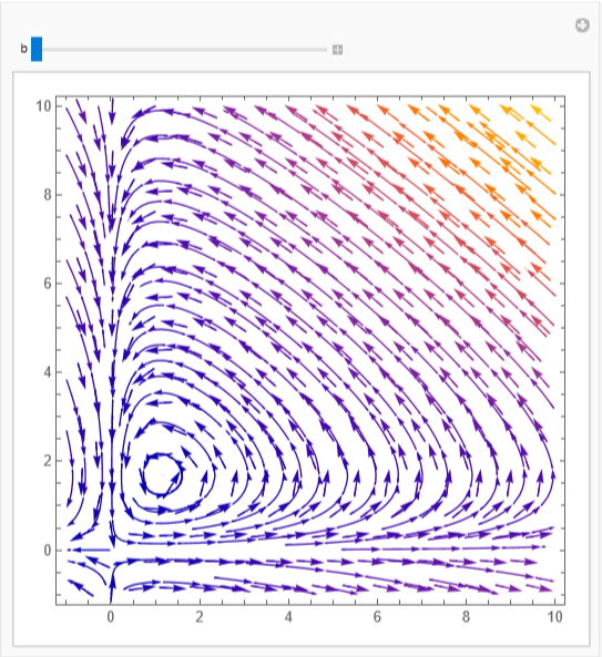
The corresponding phase portrait can be also visualized by using VectorPlot and StreamPlot. We can also put the ParametricPlot result inside this phase portrait:
In[]:=
Manipulate[Show[VectorPlot[{x*(α-βy),y*(-γ+δ*x)},{x,-1,10},{y,-1,10}],StreamPlot[{x*(α-βy),y*(-γ+δ*x)},{x,-1,10},{y,-1,10}],ParametricPlot[Evaluate[{x[t],y[t]}/.sol],{t,0,b},PlotStyle{Red,Thick}]],{b,30,50},SaveDefinitions->True]
Out[]=
The interactive visualization of solution curves
The interactive visualization of solution curves
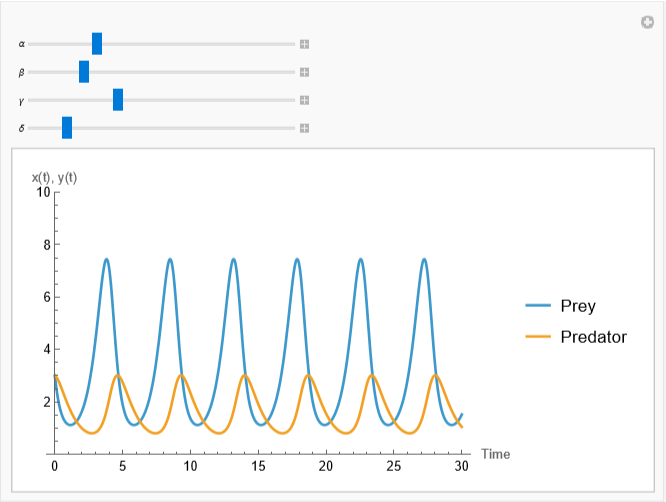
Alternatively, we can also use another built-in function ParametricNDSolve [] to create a more interactive chart of the solution curve. The ParametricNDSolve gives us the same solution curve, but it allows us to control and manipulate parameter values of the model.
With the same initial condition x(0) = 3 and y(0) = 3, we use the following syntax to generate "ParametricFunction" for each solution curve of two function variables:
In[]:=
ClearAll[α,β,γ,δ,sol,x,y,x0,y0,t];sol=ParametricNDSolve[{x'[t]==x[t]*(α-β*y[t]),y'[t]y[t]*(-γ+δ*x[t]),x[0]3,y[0]3},{x,y},{t,0,30},{α,β,γ,δ}]
Out[]=
xParametricFunction,yParametricFunction

In[]:=
Manipulate[Plot[Evaluate[{x[α,β,γ,δ][t],y[α,β,γ,δ][t]}/.sol],{t,0,30},PlotRange->{0,10},PlotLegends{"Prey","Predator"},AxesLabel{"Time","x(t), y(t)"}],{{α,2},1,5},{{β,1.2},1,2},{{γ,1},0,3},{{δ,0.3},0.1,1.6},SaveDefinitions->True]
Out[]=
A numerical example
A numerical example
The model
The model
In order to better understand the model’s dynamics, suppose that the predator-prey relationship between rabbits (x) and foxes (y) can be modeled by the following two differential equations:
As above, the population of rabbits grow exponentially by a factor of 0.1 percent in the absence of the predator. Because of its interactions with the predator, however, the rabbit’s population decreases by a factor of 0.003. On the other hand, the fox population decreases by a factor of 0.03 in the absence of its prey, rabbits. The fox population increases only when it successfully catches and feeds on rabbits.
The steady state values
The steady state values
As before, we have the following two steady state values:
The static visualization of a solution curve
The static visualization of a solution curve
The general solution of this system with the given initial condition, x(0) = 10 and y(0) = 5, can be found by the following:
We can visualize the solution curves as follows:
We can also put the parametric solution curve inside the phase portrait as before.
The static visualization of multiple solution curves
The static visualization of multiple solution curves
This time let us generate many charts showing different numerical solutions.
The interactive visualization of solution curves
The interactive visualization of solution curves
Since we are given by parameter values, let us create a slightly different interactive plot for this system, using a locator. We can define the system in the following way:
After defining a new function for the solution having the initial condition as its argument, we can use the locator as follows:
The predator-prey system with the logistic growth of the prey population
The predator-prey system with the logistic growth of the prey population
A general model
A general model
The model
The model
The previous model assumes that the prey population grows exponentially in the absence of the predator. This exponential growth of the prey population is not a realistic assumption because there is a certain natural limit imposed on the growth of the prey population even when there is no predation. In biology, this growth limit is often called the ‘carrying capacity’ of the population growth.
For example, we can think of the population of rabbits that grow rapidly in the absence of their predators. But the rabbit population cannot grow without limit because there are natural constraints typically imposed by limiting food supply. In order to account for this kind of scenario, we need to slightly modify the original predator-prey model into the following form:
where α, β, γ, δ, and n are all positive growth parameters and both x > 0 and y > 0 are the stock variables for two interacting species. The variables and parameters used in this system are the same as before. The only difference is the new term ‘x/n’ inserted in the first equation. Conceptually, the term ‘n’ represents the maximum number of the rabbit population that the surrounding natural habitat permits. As the number of rabbits reaches this limit, it plays a role as the constraining factor that affects the further growth of the rabbit population. As we will see below, the inclusion of this term substantially modify the equilibrium solution of the system and thus its dynamic behaviors.
The steady state values
The steady state values
Following the standard procedure, let us find the steady state value first:
There are two steady state equilibrium points, one of which is zero in both x and y. The value of nonzero equilibrium point is now modified from that of the previous predator-prey system. The value of the predator population near the steady state equilibrium point is also affected by the carrying capacity of the predator population.
The static visualization of a solution curve
The static visualization of a solution curve
As before, let us assign an arbitrary value to each unknown parameters and find the general solution numerically. Assuming that α = 2, β = 1.2, γ = 1, δ = 0.9, and n = 50, and the initial condition of both species x(0) = 3, y(0) = 3, let us compute the general solution and determine the property of this system.
The interactive visualization of solution curves
The interactive visualization of solution curves
Alternatively, we can also use another built-in function ParametricNDSolve to create a more interactive plot of the varying solution curve. With the same initial condition, we use the following syntax to generate “ParametricFunction” for each function of variables:
A numerical example
A numerical example
The model
The model
The following nonlinear differential equation system forms an example of the predator-prey model, in which the population of the prey species x is modeled by the logistic population growth equation. Let us find the steady state points, determine the local stability properties of each points, and draw the phase diagram.
The steady state values and local stability analysis
The steady state values and local stability analysis
We can find the following three steady state equilibrium points:
The local stability of the system near and at each steady state value can be found by taking the trace, determinant, and the eigenvalues of the Jacobian matrix of the system. If both trace and determinant are negative and the eigenvalues are all real valued negative, the corresponding steady state is a sink or attractor toward which the system converge.
For the steady state value (x, y) = (0, 0), the trace is positive and the determinant is negative, while two eigenvalues are all real valued. Therefore, this steady state point is an attractor or sink.
For (x, y) = (20, 0), the trace is positive, the determinant is negative, while the two eigenvalues are all real valued with the opposite sign. This steady state point is a source or repelling point.
Finally, for (x, y) = (50, -60), the trace is negative and the determinant is positive. The real part of two eigenvalues are negative. Therefore, this point is another attractor.
The static visualization of a solution curve
The static visualization of a solution curve
Now let us visualize the dynamics of the solution curve with the following initial conditions:
The static visualization of multiple solution curves
The static visualization of multiple solution curves
We can also run a simulation that generates various solutions behaviors depending on a number of initial conditions. For this purpose, we can build and run the following program:
The interactive visualization of solution curves
The interactive visualization of solution curves
Since we are given by parameter values, let us create a slightly different interactive plot for this system, using a locator. After defining a new function for the solution having the initial condition as its argument, we can use the locator as follows:
Interactive visualizations of the predator-prey system
Interactive visualizations of the predator-prey system
Now that we have examined a number of specifications of the predator-prey models, let us create another interactive chart that enables us to manipulate the solution curve by changing the value of parameters and initial conditions. The following demonstrations are some of these examples (Note 2).
(Note 2: Examples in this section are slightly modified versions of both Wilkerson (2011) and Weisstein (2011) )
The predator-prey system with some additional variations
The predator-prey system with some additional variations
Introduction
Introduction
In this final section, we will consider various plausible scenarios that affect the population growth of predators and preys. What would happen if humans intervene (e.g., hunting or catching) the existing biological predator-prey relations? What would happen if there is a sudden change (e.g., migration) in the population of one species? Since the population growth of one species interacts with the population growth of other species, these changes will bring corresponding nonlinear effects on the population of both species. The goal of this section is to show how to modify the original model in order to account for these likely changes in the variables and how to solve the new system (Note 3).
(Note 3: This section is inspired by Blanchard et al (2011: 20-21;162-164) and Abell and Braselton (2016: 586-593))
The starting point
The starting point
The model setting
The model setting
As a starter, let us consider the following two standard systems of predator-prey interactions:
The first system consists of two differential equations for the population growth of two species growing exponentially. In the second system, we changed the prey population growth into a logistic growth model.
The interactive solution of the system (a)
The interactive solution of the system (a)
Let us find the general solution for the first system and create an interactive plot of the solution curves.
The interactive solution of the system (b)
The interactive solution of the system (b)
The effect of hunting of the prey species
The effect of hunting of the prey species
The scenario
The scenario
Suppose that we allow hunting for the prey population. If we assume that there is a constant number of preys that is hunted by hunters. How can we modify original systems of differential equations? The effect of hunting at a rate of α unit of time is the same as the population growth of a species with constant harvesting. If we interpret this scenario as α amount of constant harvesting of the prey population, we can modify the original differential equation for the prey population as:
Now let us find the solution of the new predator-prey system with this modified equation for the prey population:
For a technical convenience, let us use an arbitrary initial condition x(0) = 1 and y(0) = 0.5.
The equilibrium points:
The solution curves for both species:
The parametric plot of two species
As the number of hunted preys (its ratio) increases, the population of the prey species decreases. But this decrease also induce the prey population decreases as well. If too much hunting of the prey species is allowed, not only the prey but also its predator species will die off. In this numerical example, the critical point of hunting ratio is α = 0.0065.
The equilibrium points:
The effect of hunting of the predator species
The effect of hunting of the predator species
The scenario
The scenario
The effect of hunting of the predator is the same as the population growth model of the predator with harvesting. Since the total number of hunting is proportional to the number of predators, we can capture this hunting rate of predators by kF where k > 0 is the constant harvesting-hunting rate parameter:
Let us now find the new solution of the system using this modified predator population equation:
The equilibrium points:
The solution curves:
The parametric plot:
As the hunting rate of the predator increases, the prey population increases in tandem.
The equilibrium points:
The solution curves:
The parametric plot:
As the hunting rate of the predator increases, the prey population increases in tandem. But because of the carrying capacity imposed on the population, the adjustment in the growth of the two population is quicker than otherwise.
The effect of the predators’ discovery of a unlimited alternative food source
The effect of the predators’ discovery of a unlimited alternative food source
The scenario
The scenario
The equilibrium points:
The solution curves:
The parametric plot:
The equilibrium points:
The solution curves:
The parametric plot:
The effect of the predators’ discovery of a limited alternative food source
The effect of the predators’ discovery of a limited alternative food source
The scenario
The scenario
The equilibrium points:
The solution curves:
The equilibrium points:
The solution curves:
The effect of the predators’ migration
The effect of the predators’ migration
The scenario
The scenario
Suppose that the predators migrate to another area if there are five times as many preys as predators in that area (that is, if x > 5y), and they move back if there are fewer than five times as many preys as predators in that area. How can we modify the system to take this into account?
The predator population in one area is now being dependent on the food availability in other area. If the condition x > 5y is satisfied in other area, the predators will move away from the original area at an immigration rate of k > 0. Therefore, we can add a term -k(x-5y) to the original differential equation for the predator population as follows:
The equilibrium points:
The solution curves:
The parametric plot:
The equilibrium points:
The solution curves:
The parametric plot:
The effect of the preys’ migration
The effect of the preys’ migration
The scenario
The scenario
Suppose now that the prey population move out from the old habitat at a rate of proportional to the number of predators in the area. How can we modify the system to take this into account? One way of doing so is to set the prey population dynamics as:
Compared to the effect of hunting, the decreasing number of the preys is now affected by the product of k and y where k > 0 is an immigration-rate coefficient, which is proportional to the number of predators.
The equilibrium points:
The solution curves:
The parametric plot:
The equilibrium points:
The solution curves:
The parametric plot:
The effect of variable growth rate coefficients due to environmental changes
The effect of variable growth rate coefficients due to environmental changes
The scenario
The scenario
Static solutions
Static solutions
Interactive solutions
Interactive solutions
Conclusion
Conclusion
In this note, we have learned how to set up and modify the classic predator-prey model and find the solution curve of the two interacting species. Starting from the original model of two nonlinear differential equations with exponential growth of the prey population, we have learned how to introduce and modify various growth factors into the model.
For example, we modified the growth of the prey population from exponential to logistic growth pattern; we have also introduced carrying capacity for both species. Finally, we have experimented with constant harvesting and migration of each species, along with some cyclical factors that affect the population growth of the prey population.
This concise presentation of the predator-prey population will be of great use in building and applying many dynamic economic and social models as well.
Reference
Reference
◼
Michael Hoy et. al ., Mathematics for Economics, MIT Press, 2022 (4th edition), pp. 907-930.
◼
Paul Blanchard, Robert L. Devaney, and Glen R. Hall, Differential Equations, Cengage Learning, 2012 (4th edition), pp.150-156.
◼
Marth L. Abell and James P. Braselton, Differential Equations with Mathematica, Elsevier and Academic Press, 2016 (4th edition), pp.565-600.
◼
Stephen Wilkerson, “Predator-Prey Model.” Wolfram Demonstration Project (2011). (https://demonstrations.wolfram.com/PredatorPreyModel/)
◼
Eric W. Weisstein, “Predator-Prey Equations., Wolfram Demonstration Project (2011) (https://demonstrations.wolfram.com/PredatorPreyEquations/)
CITE THIS NOTEBOOK
CITE THIS NOTEBOOK
Introduction to dynamic economic models: the predator-prey system
by Hee-Young Shin
Wolfram Community, STAFF PICKS, December 26, 2025
https://community.wolfram.com/groups/-/m/t/3597063
by Hee-Young Shin
Wolfram Community, STAFF PICKS, December 26, 2025
https://community.wolfram.com/groups/-/m/t/3597063