CITE THIS NOTEBOOK: Studying localization of perturbations in hypergraph evolution by Polina Blinova. Wolfram Community JAN 11 2023.
We present a study of perturbations that remain localized in the evolution of hypergraphs. In particular, we show that hyperedge reversal in pre-evolved hypergraphs leads to three types of observed behavior: rapidly-growing, contained, and non-spreading perturbations. Further, we identify classes of hypergraph rewriting rules that lead to such behaviors. It turns out that rapidly-growing hypergraphs with signature -> also generally correspond to rapidly-spreading perturbations, while rules with signature -> tend to not be affected by hyperedge reversal due to their resemblance with slowly-evolving 2D manifolds embedded in 3D space. Contained perturbations, or particle-like structures, are most rarely observed, and further research is needed to identify classes of rules that can localize such perturbations as hyperedge reversal. Our methods for comparison of hypergraph evolution in perturbed and unperturbed cases includes tracking the number and proportion of affected hyperedges over time, as well as utilizing the spectral approach to graph theory and comparing the adjacency matrices for the two cases. We are able to identify trends in spectral gaps and spectral radii that give insight into hypergraphs’ symmetry and evolution, however, further research is needed to fully understand the significance of such trends.
2
2
4
2
2
3
3
3
Contents
Contents
IntroductionII. Hyperedge reversal: general types of behaviors 2.1 Rapidly-growing perturbations Examples 2.2 Contained perturbations Examples 2.3 Non-spreading perturbations ExamplesIII. Extent of perturbation spread: adjacency matrices ExamplesIV. Rule-matching on unaffected hypergraphsV. Systematic search for rulesVI. Initialization cells with user - defined functionsConclusions and future workAppendix
I. Introduction
I. Introduction
Hyperedge reversal is one class of perturbations that can be introduced to evolving hypergraphs, and hypergraph rewriting rules with different signatures are speculated to have a different response to them. In Wolfram Physics Project, perturbations that remain localized have been denoted as “particle-like” structures, and non-planar obstructions such as and are candidates for identifying elementary particles in the Wolfram Physics Model. However, inserting nonplanarity in otherwise planar hypergraphs is not the only kind of perturbation that could remain localized over time. In this project, we investigate the effect of reversing any given hyperedge in an already pre-evolved hypergraph, and we aim to see whether there exist conditions that could force a reversed hyperedge to have a localized extent of causal influence. As an extension, we also consider matching any given hyperedge to the specified hypergraph rewriting rule.The rest of this text is structured as follows. In section II, we introduce different classes of hypergraph evolution behavior under hyperedge reversal. In section III, we analyze perturbation propagation in more details, and we utilize spectral approach to graph theory to measure and compare eigenvalues of adjacency matrices of perturbed and unperturbed graphs. In section IV, we investigate whether a different class of perturbations, namely rule-matching, has any identifiable trends as opposed to simplistic hyperedge reversal. In section V, we propose a pseudo-code for a systematic search for rules that can localize perturbations in hypergraph evolution. Section VI is devoted to all initialization cells for user-defined functions used in this project.
K
3,3
K
5
II. Hyperedge reversal: general types of behaviors
II. Hyperedge reversal: general types of behaviors
In this section, we focus on studying the reversal of hyperedges as a class of perturbations in hypergraph evolution. While there are other perturbations one could explore, such as addition/deletion of edges, most of this project will focus on hyperedge reversal. The preliminary results of such perturbations are explored in chapter 4.14 of Stephen Wolfram’s text - “A Class of Models with the Potential to Represent Fundamental Physics”.
In theory, one can reverse any given hyperedge in an already pre-evolved hypergraph. However, we speculate that the nature of perturbation chosen as well as the evolution rule matter more than the index of changed hyperedges. In light of this, the indices of hyperedges reversed in the following examples are chosen for ease of representation purposes only, and one should keep in mind that the exact details of perturbed hypergraph’s evolution would differ slightly had we opted for other hyperedges. Nevertheless, we are able to distinguish between general evolution behaviors of perturbed hypergraphs, and we separate them into 3 groups: rapidly-growing perturbations, contained perturbations, and non-spreading perturbations.
We define a function ReverseHyperedge that compares the evolution of an unperturbed hypergraph and a hypergraph with one reversed hyperedge. More detailed description as well as function definition can be found in section VI. The hypergraph plots presented in the following sections show the hyperedges that are affected by the perturbation in red (on the unperturbed hypergraph), followed by the number of affected hyperedges. We use zero initial conditions throughout.
2.1 Rapidly-growing perturbations
2.1 Rapidly-growing perturbations
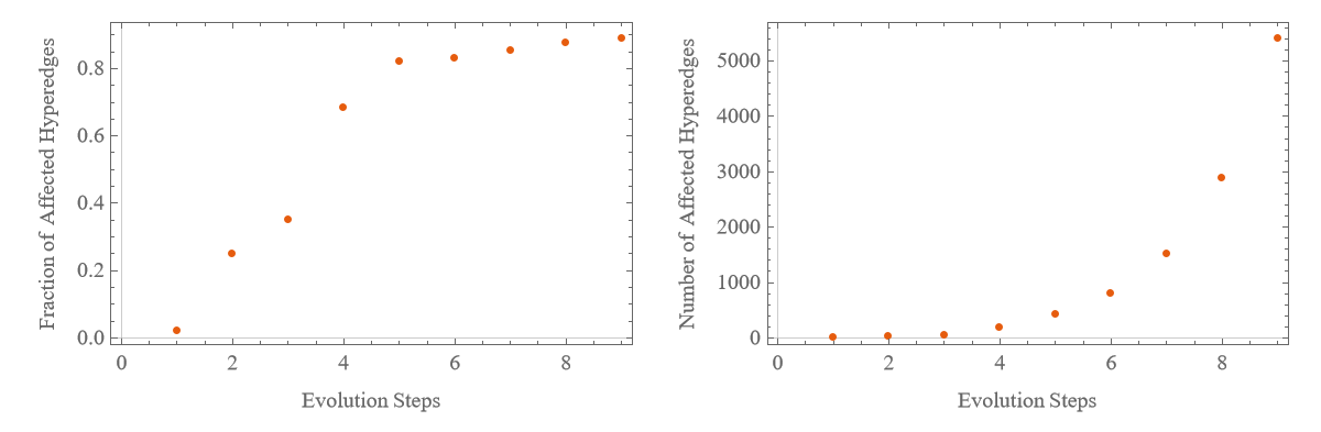
The first class of perturbed hypergraph evolution can be denoted as “rapidly-growing”. In both examples presented below, the number of affected hyperedges grows exponentially over evolution steps, and the perturbation quickly spreads through the entire structure. The examples presented here have the characteristic signature of ->, but we do not exclude the possibility that there exist other rapidly evolving hypergraphs where perturbations also spread in a “rapid” manner. In less than 1% of rules with this signature, the hypergraphs start forming “globular” structures after very few steps of evolution, and we explore some of these structures in this section [6].
In the examples given below, the hypergraphs needed to be pre-evolved to just five steps after the perturbation is introduced for the effect to propagate to more than 80% of the structure. After this point, the spread generally slows down as the number of affected hyperedges approaches 100%, which can be attributed to the slowing down in the overall growth of the hypergraph.
2
2
4
2
In the examples given below, the hypergraphs needed to be pre-evolved to just five steps after the perturbation is introduced for the effect to propagate to more than 80% of the structure. After this point, the spread generally slows down as the number of affected hyperedges approaches 100%, which can be attributed to the slowing down in the overall growth of the hypergraph.
Example 2.1.1: {{x, y}, {x, z}} {{x, z}, {x, w}, {y, w}, {z, w}}
Example 2.1.1: {{x, y}, {x, z}} {{x, z}, {x, w}, {y, w}, {z, w}}
We start with an example of the rule above and pre-evolve it to five steps. At this point, a globular structure begins forming. Eight steps later, the perturbation caused by the reversal of one hyperedge has spread to almost 100% of the hypergraph.
In[]:=
ReverseHyperedge[rule={{x,y},{x,z}}{{x,z},{x,w},{y,w},{z,w}},start={{0,0},{0,0}},edgeindex=29,steps=8,startsteps=5,incr=2]
Out[]=

We also demonstrate simple graphs that show the number/fraction of affected hyperedges over time. Note that the horizontal axis denotes evolution time steps after the perturbation is introduced. We note the exponential behaviour exhibited by the spread of the perturbation.
Out[]=
Example 2.1.2: {{x, y}, {z, y}} {{w, x}, {w, y}, {x, y}, {w, z}}
Example 2.1.2: {{x, y}, {z, y}} {{w, x}, {w, y}, {x, y}, {w, z}}
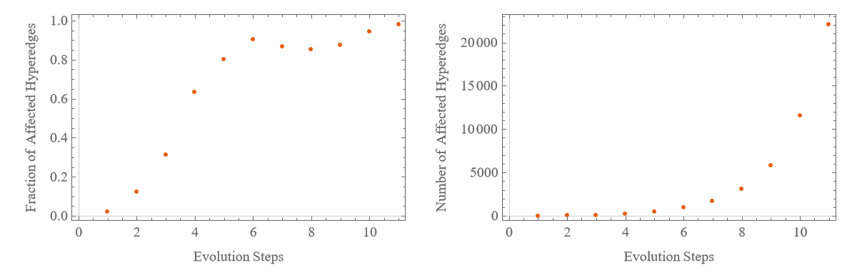
Another example of a rule with signature -> that is also pre-evolved to five steps. Again, eight steps later, the perturbation has spread to almost 100% of the structure.
2
2
4
2
In[]:=
ReverseHyperedge[rule={{x,y},{z,y}}{{w,x},{w,y},{x,y},{w,z}},start={{0,0},{0,0}},edgeindex=29,steps=10,startsteps=5,incr=2]
Out[]=

Similar graphs as above are presented. We again note the exponential behavior exhibited by the perturbation spread.
Out[]=
2.2 Contained perturbations
2.2 Contained perturbations
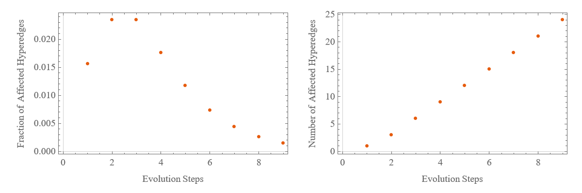
Contained or localized perturbations are another interesting class of perturbed hypergraph evolution behavior. In this case, although the number of affected hyperedges increases over time, the proportion of affected hyperedges goes down, so the perturbation stays localized. We identify two interesting examples to present here: in the first one, changes resulting from the hyperedge reversal actually stays localized, and the proportion of hyperedges affected goes to zero with evolution time steps; in the second example, the perturbation is contained at first, and then starts expanding rapidly.
Example 2.2.1: {{x, y}, {y, z}} {{w, x}, {w, y}, {x, y}, {y, z}}
Example 2.2.1: {{x, y}, {y, z}} {{w, x}, {w, y}, {x, y}, {y, z}}
This is an example of the only “truly” contained perturbation we were able to identify due to time constraints. Nevertheless, it is expected that there exist a greater number of hypergraph rewriting rules that lead to similar behavior. Although the rule has signature of ->, which we previously attributed to rapidly-growing perturbations, this example contains the perturbation to a localized spot on the hypergraph, albeit expanding rapidly itself. Note that it becomes time-consuming to run the evolution to more than 8 steps, as the number of hyperedges created grows rapidly. The figures shown are incremented by two evolution time steps each time.
2
2
4
2
In[]:=
ReverseHyperedge[rule={{x,y},{y,z}}->{{w,x},{w,y},{x,y},{y,z}},start={{0,0},{0,0}},edgeindex=30,steps=8,startsteps=5,incr=2]
Out[]=

We can also generate plots for the number and proportion of hyperedges affected with evolution steps as before. Here, it is clear that perturbation stays localized while the number of affected hyperedges increases linearly.
Out[]=
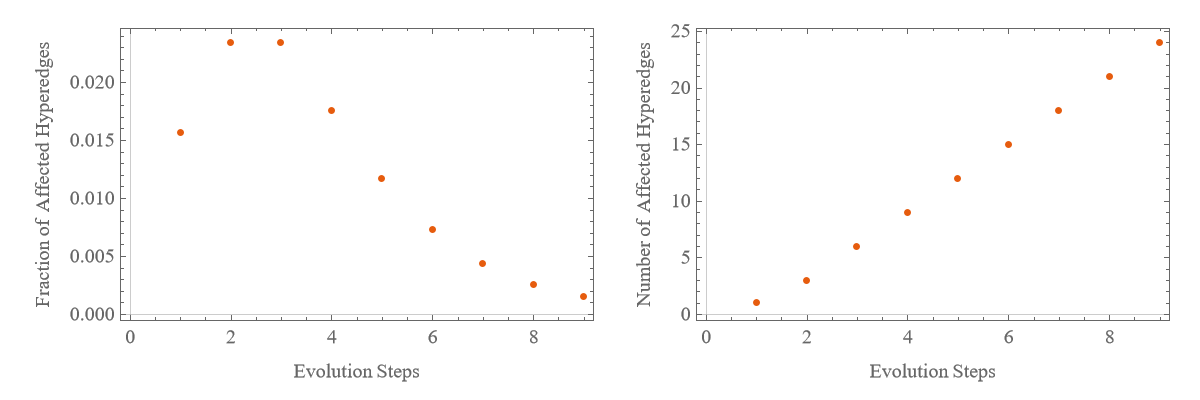
We also show that changing the initial conditions does not usually impact the localization as shown below.
In[]:=
ReverseHyperedge[rule={{x,y},{y,z}}->{{w,x},{w,y},{x,y},{y,z}},start={{1,0},{0,1}},edgeindex=30,steps=8,startsteps=5,incr=2]
Out[]=

Out[]=
Example 2.2.2: {{{x, x, y}, {z, y, u}} {{y, y, u}, {v, y, z}, {z, v, x}}}
Example 2.2.2: {{{x, x, y}, {z, y, u}} {{y, y, u}, {v, y, z}, {z, v, x}}}
This rule, also known as “wm1158”, differs slightly from the previous, but certain attributes of perturbation localization can still be traced in its evolution behavior. For the first six time steps, the perturbation does not spread, and the number of affected hyperedges remains one. This is characteristic of non-spreading perturbations explored in the next subsection. However, on time step seven, the perturbation starts expanding. Note that the figures are shown every ten evolution times steps after the hyperedge is reversed.
In[]:=
ReverseHyperedge[rule={{{1,1,2},{3,2,4}}->{{2,2,4},{5,2,3},{3,5,1}}},start={{0,0,0},{0,0,0}},edgeindex=29,steps=50,startsteps=200,incr=10]
Same plots as before showcase the containment of the perturbation on first six time steps after the hyperedge is reversed.
2.3 Non-spreading perturbations
2.3 Non-spreading perturbations
◼
Reverse the last hyperedge : evolution stops because the only relation that matches the left - hand side of the rule is changed. Note that if a symmetric hyperedge is reversed, the growth can theoretically continue, but we discard these types of perturbations since they do not actually change any existing relations in the hypergraph.
◼
Reverse any other hyperedge : the affected hyperedge stays in the same place . No propagation is observed because simple hyperedge reversal somewhere in the middle of the pre - evolved hypergraph is not sufficient to guarantee that the perturbed hypergraph will match the rule in more than one place (outer two hyperedges).
Below, we present examples of hyperedge reversal in such globular structures. More examples of similar rules can be found in sections 3.10 and 4.1 of Stephen Wolfram's text - "A Class of Models with the Potential to Represent Fundamental Physics".
Example 2.3.1: {{x, y, y}, {z, x, u}} {{y, v, y}, {y, z, v}, {u, v, v}}
Example 2.3.1: {{x, y, y}, {z, x, u}} {{y, v, y}, {y, z, v}, {u, v, v}}
Example 2.3.2: {{x, y, z}, {u, y, v}} {{w, z, x}, {z, w, u}, {x, y, w}}
Example 2.3.2: {{x, y, z}, {u, y, v}} {{w, z, x}, {z, w, u}, {x, y, w}}
Example 2.3.3: {{x, x, y},{x, z, u}} {{u, u, z},{y, v, z},{y, v, z}}
Example 2.3.3: {{x, x, y},{x, z, u}} {{u, u, z},{y, v, z},{y, v, z}}
Example 2.3.4: {{x, x, y},{z, u, y}} {{u, u, y},{x, v, y},{x, v, z}}
Example 2.3.4: {{x, x, y},{z, u, y}} {{u, u, y},{x, v, y},{x, v, z}}
III. Extent of perturbation spread: adjacency matrices
III. Extent of perturbation spread: adjacency matrices
As another way to characterize the extent of perturbation (i.e. compare the evolution of perturbed and unperturbed hypergraphs), we propose to make use of adjacency matrices. An adjacency matrix for a directed graph is defined as follows [1][5]:
Technically, we would need to resort to an adjacency tensor in this case, but Wolfram function repository has a defined function that converts a hypergraph’s adjacency tensor into an adjacency matrix. In this project, we propose to compare the perturbed and unperturbed hypergraphs by their respective spectra (sets of eigenvalues for the adjacency matrices of graphs). More precisely, eigenvalues are the sets of scalars such that:
Example 2.1.2: rapidly-growing perturbations
Example 2.1.2: rapidly-growing perturbations
Conducting the spectral analysis for the two examples of rapidly-evolving perturbations introduced above yielded all eigenvalues of the adjacency matrices for both unperturbed and perturbed hypergraphs to be zero. For convenience, we only show results of analysis for the hypergraph evolution shown above.
Example 2.2.1: contained perturbations
Example 2.2.1: contained perturbations
We conduct the spectral analysis of the hypergraph evolution shown above. Eigenvalues do not match, so the graphs are not isomorphic, which is to be expected [2]. Below, the visualization of eigenvalue trends over evolution steps is presented.
From the graph above, it can be noticed that eigenvalues of the adjacency matrices do not change over time. Particularly, the spectral gap and the spectral radius are also constant, which is shown below. This indicates that the eigenvalues of the adjacency matrix do not evolve significantly after the perturbation is introduced. We speculate that this has to do with the fact that the perturbation is localized and does not spread.
We note that the spectral gap is higher for the unperturbed hypergraph, which could indicate that its expansion is higher compared to when one hyperedge is reversed [3][4]. On the other hand, the spectral radius is higher for the perturbed hypergraph.
Example 2.3.2: non-spreading perturbations
Example 2.3.2: non-spreading perturbations
We conduct the spectral analysis of the hypergraph evolution shown above. Below, the visualization of eigenvalue trends over evolution steps is presented.
Although the specific eigenvalues differ from one evolution step to another, a notable characteristic for all evolution steps is the large difference between the second and leading eigenvalues of the adjacency matrices. A more detailed example comparing the evolution one step and 40 steps after the reversal of a hyperedge is introduced. Measurement of spectral gap is the metric that changes most drastically of those explored
The following plot shows spectral gap differences for adjacency matrices on different steps in evolution (horizontal axis) of perturbed and unperturbed hypergraphs. The overall trend indicates that spectral gap decreases over time. While the two trends move together, it is not possible to say whether the spectral gap for the perturbed or the unperturbed hypergraph is greater on average.
Spectral gap is linked to graph’s expansion [3][4]. On these grounds, we speculate that the hypergraph’s expansion is higher at the beginning of evolution. Intuitively, this makes sense, as hypergraphs that can form “globular structures” exhibit slower growth (in terms of the number of hyperedges added to the total number of hyperedges existing), as times goes on. Since, both unperturbed and perturbed hypergraphs follow the same trend for spectral gaps and radii, this may be an indicator that hyperedge reversal does not lead to any significant changes propagating through these hypergraphs.
Spectral gap is linked to graph’s expansion [3][4]. On these grounds, we speculate that the hypergraph’s expansion is higher at the beginning of evolution. Intuitively, this makes sense, as hypergraphs that can form “globular structures” exhibit slower growth (in terms of the number of hyperedges added to the total number of hyperedges existing), as times goes on. Since, both unperturbed and perturbed hypergraphs follow the same trend for spectral gaps and radii, this may be an indicator that hyperedge reversal does not lead to any significant changes propagating through these hypergraphs.
We note that the spectral radius is usually greater for the unperturbed graph than for the perturbed. We state this as an observation, and more research is needed to understand the nature and significance of this fact.
IV. Rule-matching on unaffected hypergraphs
IV. Rule-matching on unaffected hypergraphs
However, we can artificially force some of the previously created hyperedges to match the left-hand side of the rule, in which case the propagation of the perturbation will be seen. We define a function MatchHyperedge for this purpose.
Looking at how the proportion and number of hyperedges affected over time changes, one notes the rapid increase for the first ten steps after the perturbation is introduced, and then a linear and steady increase. However, depending on which hyperedge is perturbed, one could get a completely different trend, and more research is needed to identify any generalities.
The evolution itself looks like the following. The structure barely resembles the unperturbed graph after a couple evolution steps.
In general, one can get rather unpredictable behavior when matching a rule for a random hyperedge. For instance, the hypergraph could become disconnected like in the following example, where edge number 29 is matched to the rule:
Here is another example of a rule that was not affected by a reversed hyperedge. Again, forcing any given hyperedge to match the left-hand side of the rule can yield rather interesting results. Below, one can notice that the hypergraph forms a “tail” that is not observed in the original case.
Below is the evolution of the perturbed hypergraph. On these grounds, we can speculate that the combination of a perturbation and the rule affects the evolution more than any parameter individually.
V. Systematic search for rules
V. Systematic search for rules
We attach a pseudo code for a systematic search of rules that localize introduced perturbations for further research. Due to time constraints, we are not able to implement it yet, but this is a great alley to expand upon our findings in this domain of research.
Concluding remarks
Concluding remarks
Appendix
Appendix
I would like to thank John McNally for defining all of the following functions used in the appendix and for formulating the examples that open a new way to develop this project.
We have explored only hyperedge reversal and rule-matching as perturbations in this text. However, it would be useful to define a function to introduce any perturbation that the user can define:
We have explored only hyperedge reversal and rule-matching as perturbations in this text. However, it would be useful to define a function to introduce any perturbation that the user can define:
This can also allow us to check if our initial speculation that the index of the hyperedge reversed does not impact the overall evolution trend is true.
We can start noticing some differences on the second step already. Perhaps, the index of the reversed hyperedge matters more than was originally assumed. We can go through every possible scenario and make a grid of our results. Note that we are only tracking the evolution for two steps here and showing the first four rows of the grid. For full analysis, one should run the code for all the hyperedges.
First we check the total number of hyperedges:
First we check the total number of hyperedges:
And then we form a grid with every single hyperedge perturbed individually (only first four rows shown):
And then we form a grid with every single hyperedge perturbed individually (only first four rows shown):
In general, we can define a function that counts the number of hyperedges that are affected over time (i.e. in the perturbed state but not in the unperturbed one).
We can also try visualizing how the number of affected hyperedges changes over time depending on which hyperedge we perturb.
For instance, the rule that was speculated to localize the perturbations (example 2.2.1), turns out to do so only upon reversal of certain hyperedges. Apparently, there exist other hyperedges that cause the perturbation to propagate through the entire hypergraph. Here we are only showing the reversal of the first four hyperedges.
This shows that there exist many more topics for exploration that we only briefly touched upon in this text. Our findings are only preliminary, and there remains much more to be explored in this area.
Keywords
Keywords
◼
Perturbation
◼
Hypergraph
◼
Adjacency Matrix
◼
Spectral Approach
Acknowledgment
Acknowledgment
I would like to extend my gratitude to Stephen Wolfram for focusing this research project and suggesting the idea of identifying localized perturbations in hypergraph evolution. I would also like to thank Simon Fischer and John McNally for their excellent supervision and guidance. Their advice, suggestions, and coding help were invaluable. Furthermore, I want to thank Xerxes D. Arsiwalla for suggesting the idea of computing top eigenvalues of hypergraph’s adjacency matrices as a more formal way to compare perturbed and unperturbed cases. Finally, I want to thank everyone who made Wolfram Winter School possible.
References
References
◼
[1] Adjacency matrix. (n.d.). Retrieved January 11, 2023, from https://mathworld.wolfram.com/AdjacencyMatrix.html#:~:text=The %20 adjacency %20 matrix %2 C %20 sometimes %20 also,have %200 s %20 on %20 the %20 diagonal.
◼
[2] Butler, S. K. (2008). Eigenvalues and Structures of Graphs (Unpublished doctoral dissertation). University of California, San Diego.
◼
[3] Hoory, S., Linial, N., & Wigderson, A. (2006). Expander graphs and their applications. Bulletin of the American Mathematical Society, 43(04), 439-562. doi:10.1090/s0273-0979-06-01126-8
◼
[4] Raghavendra, P., & Steurer, D. (2010). Graph expansion and the unique games conjecture. Proceedings of the Forty-second ACM Symposium on Theory of Computing. doi:10.1145/1806689.1806792
◼
[5] What is an adjacency matrix - javatpoint. (n.d.). Retrieved January 11, 2023, from https://www.javatpoint.com/what-is-an-adjacency-matrix
◼
[6] Wolfram, S. (2020). A class of models with the potential to represent fundamental physics. Complex Systems, 29(2), 107-536. doi:10.25088/complexsystems.29.1.2