ABSTRACT (original article): We present an exact analytical solution of the periodic time-dependent thermo-viscoelastic problem for the infinite half space with traction-less surface and a volume heat source arising from laser penetration. We take into account the extension of the heat source, the mutual dependence of heat transfer and elasticity and the viscosity of the material, to describe damping of elastic waves, and in particular surface waves for periodic driving. The solution of the heat equation (including temperature change caused by compression/dilatation of the material) is also provided and a numerical example for aluminium, where this is demonstrated, is given. CITATION (original article): Wenin, M. Exact solution of the coupled thermo–viscoelastic problem for the semi-infinite space. Appl. Phys. A 131, 295 (2025). https://doi.org/10.1007/s00339-025-08422-0
Introduction
Introduction
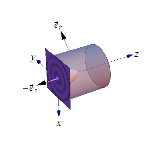
We consider a homogeneoues material in semi - infinity space. A laser points at the surface, representing a periodically driven volume heat source. The cylindrically symmetrical problem means finding the temperature and the displacement field, where we use classical continuum mechanics/physics [1,2]. Details of the analytical calculations are given in [3], which also contains a Mathematica notebook (supplementary matertial) with the analytical proofs. Here we use the formulas for numerical computations. Because the large number of material parameters in this problem, this notebook can represent only a snapshot of possible explorations. We start with the equation of motion for the displacement vector u(r,z,t), given by (ρ is the density of the material)∇·σ =ρ u,where the stress tensor σ contains three parts,σ = + + , = elastic stress tensor, = viscosity tensor,=K (T-) 1 thermal stress tensor, with: 1 the unity matrix, K modulus of compressibility, thermal volume expansion coefficient, temperature of the sample. Furthermore we use the heat equation for the temperature T(r,z,t):T- = ∇·u,with: α thermal diffusivity, q(r,z,t) laser heat source and k thermal conductivity, respectively. All calculations are performed in cylindrical coordinates {r,ϕ,z}, without ϕ - dependency. Boundary conditions: σ·n = 0, n = - , stress free surface, =0, no heat current at the surface. One derives two wave equations for longitudinal and transverse waves. We introduce Fourier transformed quantities: u = , T = , and obtain two Helmholtz equations for the displacement fields. We split the quantities “temperature” and “displacement” into two parts, corresponding to the two sources in the heat equation (inhomogeneities on the r.h.s) = + δ, = + δ. The “q - quantities” correspond to the laser source (first source) and the “δ - quantities” to the compression/dilatation process (second source). One can assume >> δ, >> δ. Evaluation of the notebook takes a few minutes.
2
∂
∂
2
t
σ
el
σ
visc
σ
T
σ
el
σ
visc
σ
T
α
T
T
0
α
T
T
0
2
∇
1
α
∂T
∂t
-q+
1
k
Kα
k
e
z
(∂T/∂z)
z=0
u
ωt
T
ωt
u
u
q
u
T
T
q
T
u
q
u
T
q
T
ClearAll["Global`*"]SetOptions[Plot,{BaseStyle{FontSize12},FrameTrue}];SetOptions[ListLinePlot,{BaseStyle{FontSize12},FrameTrue}];
Mechanical properties of Al
Mechanical properties of Al
Mechanical properties are: adiabatic modulus of compressibility, adiabatic shear modulus, adiabatic Poisson number, adiabatic modulus of elasticity, density, parameters of viscosity. We introduce longitudinal and transverse complex speeds of sound.
Kp=75.210^9;(*moduluscompress.Pa*)μs=26.310^9;(*shearmodulusPa*)σpoiss=(3Kp-2μs)/(2(3Kp+μs));(*Poissonnumber*)El=2μs(1+σpoiss);(*modulusofelasticity*)ρ=2700;(*densitykg/m^3*)ηd=10000;(*shearviscosity,ηd/1000correspondskg/(m*s)*)ζd=0;(*volumeviscosity;*)cl0=;(*speedofsound,long.*)ct0=;(*speedofsound,transv.*)cl[ω_,η_,ζ_]:=
El(1-σpoiss)
ρ(1+σpoiss)(1-2σpoiss)
μs
ρ
cl0^2+Iω(4η/3+ζ)/ρ
;(*complexspeedofsound,long.m/s,ormm/ms*)ct[ω_,η_]:=ct0^2+Iωη/ρ
;(*complexspeedofsound,transv.m/s*)Thermal properties of Al
Thermal properties of Al
In[]:=
αT=3*23.510^-6;(*coefficientofthermalexpansion1/K*)cv=900;(*heatcapacityJ/kgK*)ktherm=237;(*thermalconductivityW/mK*)α=10^3ktherm/(ρcv);(*thermaldiffusivitymm^2/ms*)μd=10^6;(*absorbtioncoefficientin1/mm*)
T0=293;(*Temperaturesample*)Tv=-αTT0Kp/(ρcv);(*auxiliaryquantity,unitK*)
Properties of the laser
Properties of the laser
In[]:=
ω0=10000;(*angularfrequencyinkHz*)tν=(2Pi/ω0);(*periodinms*)Δr=0.5;(*beamradiusinmm*)I0=10^5;(*intensityW/mm^2*)R=0.988;(*reflectioncoeff.,for>1μmwavelength*)
Characterization of the heat source
Characterization of the heat source
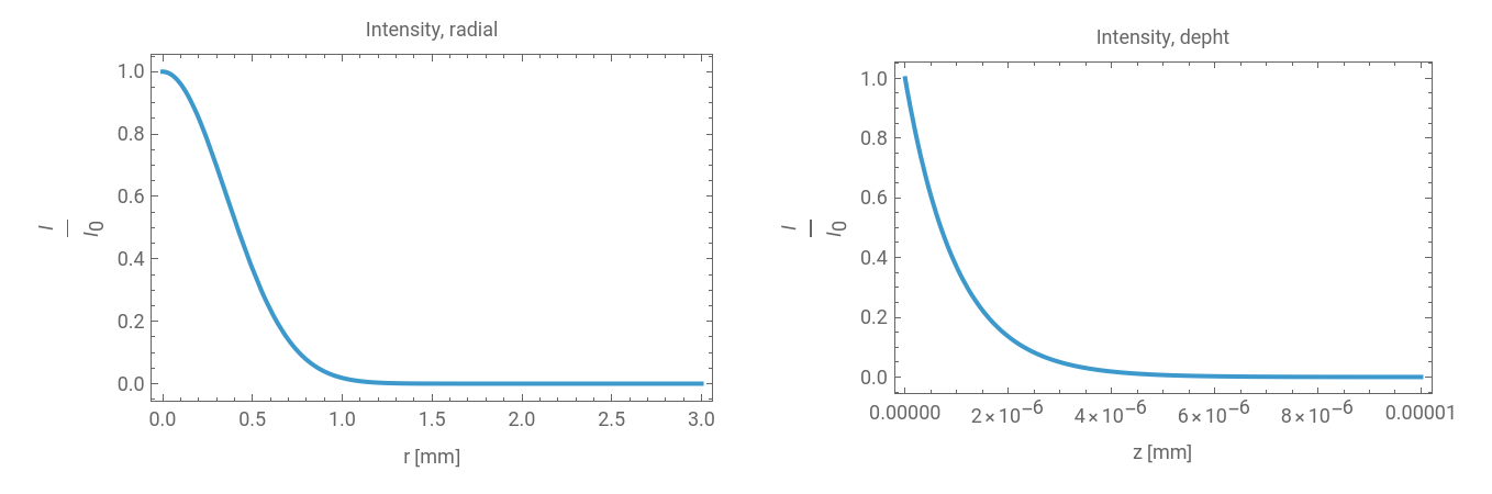
GraphicsRowPlotExp[-(r/Δr)^2],{r,0,3},FrameLabel"r [mm]","","Intensity, radial",PlotRangeAll,PlotExp[-μdz],{z,0,10/μd},FrameLabel"z [mm]","","Intensity, depht",PlotRangeAll,ImageSize->700
I
I
0
I
I
0
Out[]=
First heat source (laser)
First heat source (laser)
The laser represents the main heat source inside the material. One can say, this is a local heat source. The temperature distribution and the displacement field are given as integrals, which we solve numerically. The problem is coupled in one direction only, temperature ⟶ displacement.
Temperature distribution
Temperature distribution
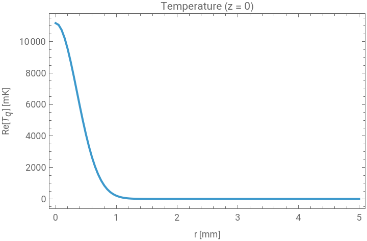
We take the formulas from [2]. Numerical evaluation of the integral to compute the temperature as a function of depht and radius.
In[]:=
ζn[λ_,ω_]:=Sqrt+;(*1/mm,whereωinkH*)(*TinmK*)T[z_?NumericQ,r_?NumericQ,ω_?NumericQ,μ_?NumericQ]:=10^6**NIntegrate-*Exp[-ζn[λ,ω]z]-Exp[-μz],{λ,0,250/Δr},Method{Automatic,"SymbolicProcessing"0},WorkingPrecision12,AccuracyGoal8,MinRecursion9,MaxRecursion12tabTq=ParallelTable[{r,T[0,r,ω0,μd]//Re},{r,0,5,0.05}];ListLinePlot[tabTq,FrameLabel{"r [mm]","Re[] [mK]"},PlotLabel->"Temperature (z = 0)",PlotRangeAll]
2
λ
Iω
α
μ*(1-R)*I0*Δr^2
2ktherm
λExp[-(λΔr/2)^2]BesselJ[0,λr]
2
μ
2
ζn[λ,ω]
μ
ζn[λ,ω]
T
q
Out[]=
Displacement field
Displacement field
The computation of the displacements requires some preliminaries (see [3]).
Damping causes (frequency dependent) complex velocities for all wave modes
Plot of integral kernels, used to compute the displacement
Computation of the displacement (last step: numerical integration over λ)
Plot of the solution on the surface
Plot of the solution on the surface
Trajectory in space of a mass element (Lagrange picture)
Trajectory in space of a mass element (Lagrange picture)
Surface waves are not pure longitudinal or transverse waves, but represent more complicated motion processes (Rayleigh waves, [1]), especially when thermal dilation is taken into account.
Second heat source (compression/dilatation of the material)
Second heat source (compression/dilatation of the material)
Setup of the solution, assignment of numerical values
Setup of the solution, assignment of numerical values
Auxiliary quantities
Homogeneous solutions
Some auxiliary quantities
Inhomogeneous solutions
Final expressions to compute the temperature and the displacement fields for the second heat source
Final expressions to compute the temperature and the displacement fields for the second heat source
Finally, we have for the temperature for the second source (integration over λ)
Final expressions to calculate the displacement field for the second source (integration over λ)
Plot of the fields
Plot of the fields
Temperature on the surface
Displacement on the surface
References
References
[1] L. D. Landau und E. Lifschitz, Lehrbuch der Theoretischen Physik VII, Elastizitätstheorie, Verlag Harry Deutsch (2007)
[2] A. Mandelis, Diffusion - Wave fields (Springer 2001)
[3] M. Wenin, Exact solution of the coupled thermo – viscoelastic problem for the semi - infinite space, Appl. Phys. A, 131, 295 (2025)
CITE THIS NOTEBOOK
CITE THIS NOTEBOOK
Exact solution of the coupled thermo - viscoelastic problem for the semi - infinite space
by Markus Wenin
Wolfram Community, STAFF PICKS, April 11, 2025
https://community.wolfram.com/groups/-/m/t/3443329
by Markus Wenin
Wolfram Community, STAFF PICKS, April 11, 2025
https://community.wolfram.com/groups/-/m/t/3443329