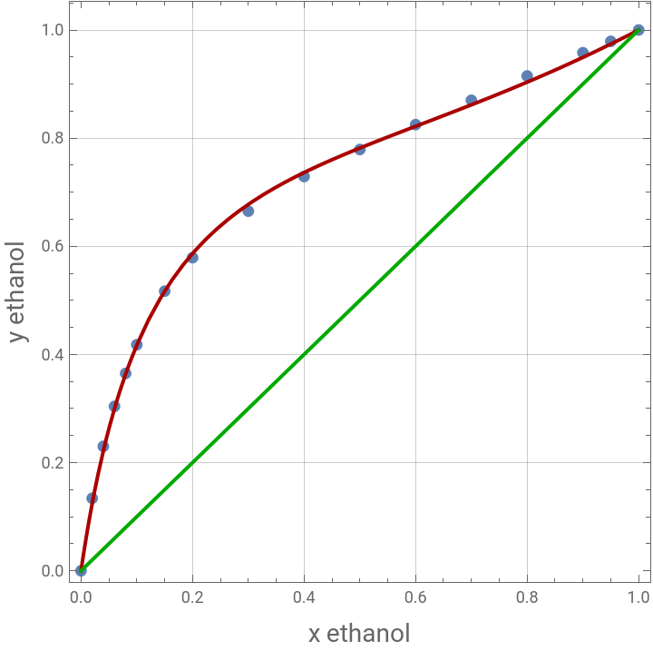
In many calculations, it is handy to have a simple equation describing VLE data (x-y relations) of non-ideal mixtures. One particular equation have been presented by Doherty and Malone in Ref. 1 and is given by: where a and b are to be determined using some curve fitting technique.
y=+bx(1-x)
ax
(1+(a-1)x)
The above relation applies only to:1- Mixture with positive azeotropes (minimum boiling azeotropes)2- Mixture with inflections but no azeotropes3- Mixture without inflections or azeotropesHence, this equation is not valid for mixture with negative azeotropes. It should be noted that this is not a serious limitation since maximum boiling azeotropes are very scares compared to other non-ideal mixtures. In the present notebook, we show how one can quickly and accurately reproduce Table 2.6 page 42 of Ref. 1. Three illustrations are presented corresponding to the different non-ideal mixtures covered by this x-y equation.
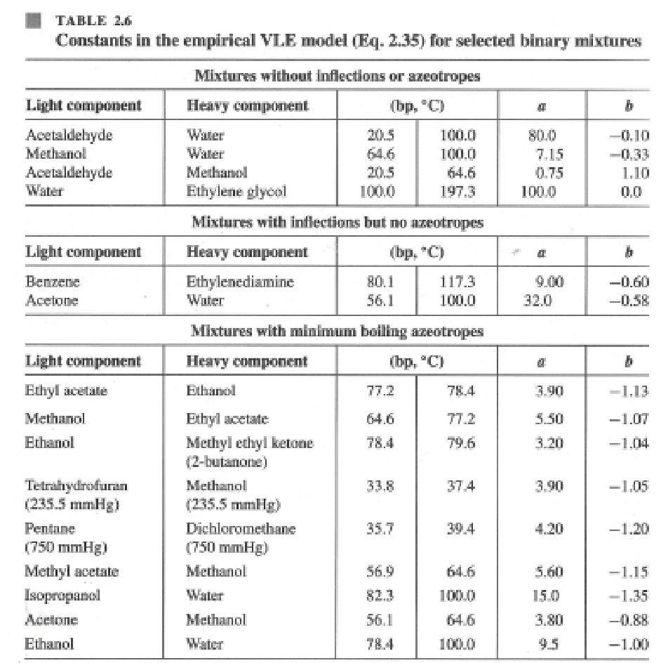
Illustration 1 : Mixture with positive azeotropes (minimum boiling azeotropes). Vapor - Liquid equilibrium data for ethanol and water at 1 atm by [2].
In[]:=
DATAEW={{0.,0.},{0.019,0.17},{0.0721,0.3891},{0.099,0.4375},{0.1238,0.4704},{0.1661,0.5089},{0.2337,0.5445},{0.2608,0.558},{0.3273,0.5826},{0.3965,0.6122},{0.5198,0.6599},{0.5732,0.6841},{0.6763,0.7385},{0.7472,0.7815},{0.8943,0.8943},{1.,1.}};
In[]:=
nlm=NonlinearModelFit[DATAEW,ax/(1+(a-1)x)+bx(1-x),{a,b},x]
Out[]=
FittedModel
In[]:=
Normal[nlm]
Out[]=
-1.05591(1-x)x+
10.0652x
1+9.06521x
In[]:=
nlm["RSquared"]
Out[]=
0.999505
In[]:=
nlm["ParameterTable"]
Out[]=
Estimate | Standard Error | t-Statistic | P-Value | |
a | 10.0652 | 0.341218 | 29.4979 | 5.2658× -14 10 |
b | -1.05591 | 0.0308614 | -34.2147 | 6.77904× -15 10 |
Experimental : blue dots and Predicted : Red curve
In[]:=
Show[ListPlot[DATAEW,PlotStyle{PointSize[0.02]}],Plot[nlm[x],{x,0,1},PlotStyle{Thick,Darker@Red}],FrameTrue,FrameLabel{Style["x ethanol",14],Style["y ethanol",14]},GridLinesAutomatic,AspectRatio1,Epilog{Darker@Green,Thick,Line[{{0,0},{1,1}}]}]
Out[]=
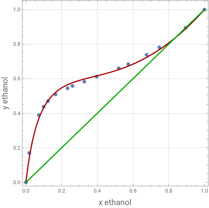
Illustration 2 : Mixture with inflections but no azeotropes. Vapor - Liquid equilibrium data for acetone and water at 1 atm by [3].
In[]:=
DATAAW={{0,0},{0.05,0.6381},{0.1,0.7301},{0.15,0.7716},{0.2,0.7916},{0.3,0.8124},{0.4,0.8269},{0.5,0.8387},{0.6,0.8532},{0.7,0.8712},{0.8,0.895},{0.9,0.9335},{0.95,0.9627},{1,1}};
In[]:=
nlm=NonlinearModelFit[DATAAW,ax/(1+(a-1)x)+bx(1-x),{a,b},x]
Out[]=
FittedModel
In[]:=
Normal[nlm]
Out[]=
-0.574272(1-x)x+
34.6367x
1+33.6367x
In[]:=
nlm["RSquared"]
Out[]=
0.999846
In[]:=
nlm["ParameterTable"]
Out[]=
Estimate | Standard Error | t-Statistic | P-Value | |
a | 34.6367 | 1.3014 | 26.6149 | 4.85562× -12 10 |
b | -0.574272 | 0.0208201 | -27.5826 | 3.1835× -12 10 |
Experimental : blue dots and Predicted : Red curve
In[]:=
Show[ListPlot[DATAAW,PlotStyle{PointSize[0.02]}],Plot[nlm[x],{x,0,1},PlotStyle{Thick,Darker@Red},PlotRangeAll],FrameTrue,FrameLabel{Style["x acetone",14],Style["y acetone",14]},GridLinesAutomatic,AspectRatio1,Epilog{Darker@Green,Thick,Line[{{0,0},{1,1}}]}]
Out[]=
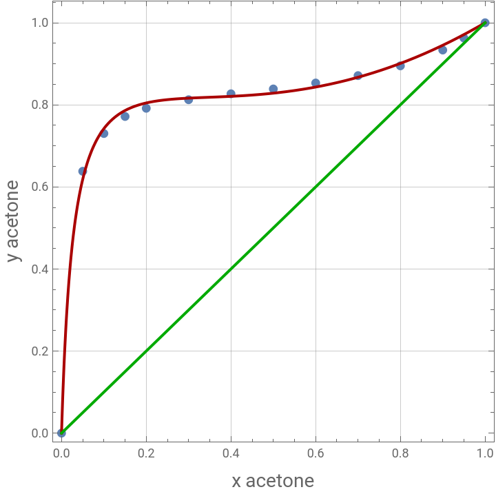
Illustration 3 : Mixture without inflections or azeotropes. Vapor - Liquid equilibrium data for methanol and water at 1 atm by 1 atm by [2].
In[]:=
DATAMW={{0,0},{2.,13.4},{4.,23.},{6.,30.4},{8.,36.5},{10.,41.8},{15.,51.7},{20.,57.9},{30.,66.5},{40.,72.9},{50.,77.9},{60.,82.5},{70.,87.},{80.,91.5},{90.,95.8},{95.,97.9},{100.,100.}}/100;
In[]:=
nlm=NonlinearModelFit[DATAMW,ax/(1+(a-1)x)+bx(1-x),{a,b},x]
Out[]=
FittedModel
In[]:=
Normal[nlm]
Out[]=
-0.399993(1-x)x+
7.45106x
1+6.45106x
In[]:=
nlm["RSquared"]
Out[]=
0.9999
In[]:=
nlm["ParameterTable"]
Out[]=
Estimate | Standard Error | t-Statistic | P-Value | |
a | 7.45106 | 0.118148 | 63.0652 | 1.3151× -19 10 |
b | -0.399993 | 0.0165911 | -24.1089 | 2.07279× -13 10 |
Experimental : blue dots and Predicted : Red curve
In[]:=
Show[ListPlot[DATAMW,PlotStyle{PointSize[0.02]}],Plot[nlm[x],{x,0,1},PlotStyle{Thick,Darker@Red}],FrameTrue,FrameLabel{Style["x ethanol",14],Style["y ethanol",14]},GridLinesAutomatic,AspectRatio1,Epilog{Darker@Green,Thick,Line[{{0,0},{1,1}}]}]
Out[]=
References
References
◼
[1] M.F.Doherty and M.F.Malone, Conceptual Design of Distillation Systems, Boston : McGraw - Hill, 2001.
◼
[2] A. K. Coker. R. H. Perry, C. H.Chilton and S.O.Kirkpatrick (Eds.), Chemical Engineering Handbook, 4th ed. New York: McGraw - Hill, p 13 - 5, 1963
◼
[3] M. F. Doherty et al. D. W. Green and R.H.Perry (Eds.), Chemical Engineering Handbook, 8th ed. New York: McGraw - Hill, p 13 - 7, 2007
CITE THIS NOTEBOOK
CITE THIS NOTEBOOK
Constants of Empirical Vapor-Liquid Equilibrium Model
by Housam Binous and Ahmed Bellagi
Wolfram Community, STAFF PICKS, February 7, 2024
https://community.wolfram.com/groups/-/m/t/3117579
by Housam Binous and Ahmed Bellagi
Wolfram Community, STAFF PICKS, February 7, 2024
https://community.wolfram.com/groups/-/m/t/3117579