Wolfram Cloud Document

Introduction

A number of years ago I came across a promotional feature within the 888 Poker app. It was called Card Strike, and it was essentially a ‘side game’ played concurrently with cash games. The rules are outlined in this short, ostentatious video, and on this website, but I will list them here as well.

◼

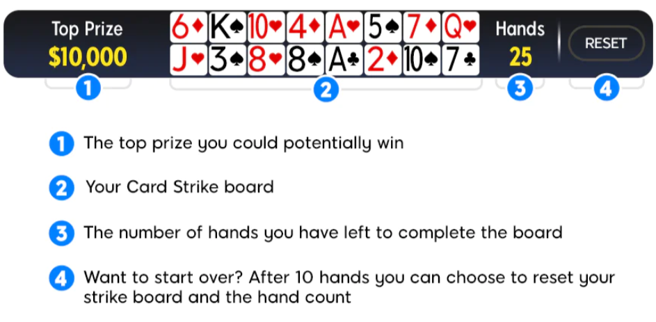
When you ‘take a seat’ at an ordinary cash game table or a SNAP cash game table, 16 random cards appear at the top of your screen. I will refer to these cards as target cards.

◼

SNAP poker is a fast format in which you are seated at a new table, and dealt a new hand, as soon as you fold.

◼

Once you are dealt your ‘hole cards’ they are checked against the target cards and if any of them match, then the appropriate target card(s) are ‘struck’.

◼

There is also a hand limit which shows the number of hands remaining for you to ‘strike’ all of the target cards.

◼

You are able to reset your target cards and hand limit, thereby starting over, after ten hands have been played.

◼

If you are successful, you are given the opportunity to spin a wheel for random cash prize determined by the stakes of the cash game. It looks like the maximum prize is $10,000, however this is likely in a ‘high stakes’ cash game already.

Simple enough! What’s more is that it is completely free, and requires no skill. You are at the probabilistic whims of the cards you are dealt.

I thought that this presented a good opportunity to explore the statistics of this game, and perhaps stumble upon some interesting results.

From: https://www.888poker.com/poker-promotions/card-strike/

Disclaimer

Gambling involves financial risk and can be addictive. The content in this article is provided for educational and analytical purposes only and should not be interpreted as encouragement to gamble. Always play responsibly, set clear limits, and seek help if you believe you may have a gambling problem. For confidential advice and support in the UK, contact GamCare at gamcare.org.uk or call 0808 8020 133.

One Hand at a Time

I will start by exploring the probabilities of all possible Card Strike-related events for a given hand of Texas Hold ‘em (also available for Pot Limit Omaha, which I won’t discuss here).

Each hand you receive 2 distinct hole cards from a 52-card deck. Therefore, you could strike 2, 1, or 0 target cards. I will write functions for each case, assuming k target cards. It is my understanding that, initially, k is equal to 16.

In[]:=

Clear[p0,p1,p2];p0[k_]:=

Binomial[52-k,2]

Binomial[52,2]

;p2[k_]:=Ifk>=2,

Binomial[k,2]

Binomial[52,2]

,0;p1[k_]:=1-p0[k]-p2[k];

Transition Matrix

We can think of the number of target cards remaining as our ‘state’. The probability of getting to the next ‘state’ depends only on the current ‘state’ and not on the history of how we got there. This setup lends itself to a Markov transition matrix.
“Interestingly, Markov chains have historical ties to processes like card shuffling. My goal is to show how these mathematical tools and techniques are not so scary, especially if you can harness the power of Wolfram Language.

For 16 target cards, there are 17 possible discrete states (k = 16 to k = 0). Each time you play a hand, there is some probability that you transition to a new state where k has reduced by 2, 1, or has stayed the same.
It is helpful to reformulate in terms of the number of cards actually struck (ψ = 16 - k), which can range from ψ = 0 to ψ = 16, since this allows us to ‘start’ in the top-left of our matrix and work our way downwards and rightwards as we reach the end.
When setting up our transition matrix P, we will use the following rules:

◼

Element

ψ,ψ

represents the probability of striking 0 target cards. For example

(1st row, 1st column) represents the probability that ψ remains at 0.

◼

Element

ψ,ψ+1

represents the probability of striking exactly 1 target card. For example

(1st row, 2nd column) represents the probability that ψ goes from 0 to 1.

◼

Element

ψ,ψ+2

represents the probability of striking 2 target cards. For example

(1st row, 3rd column) represents the probability that ψ goes from 0 to 2.

◼

All other entries are 0, since you cannot strike more than 2 cards per hand, nor ‘un-strike’ target cards.

I will create this matrix with the help of SparseArray and Band, defining

as the initial number of target cards.

In[]:=

k0=16;P=SparseArray[{Band[{1,1}]->Table[p0[k0-ψ],{ψ,0,k0}],Band[{1,2}]->Table[p1[k0-ψ],{ψ,0,k0-1}],Band[{1,3}]->Table[p2[k0-ψ],{ψ,0,k0-2}]},{k0+1,k0+1}];MatrixForm[P]

Out[]//MatrixForm=

105 221	96 221	20 221	0	0	0	0	0	0	0	0	0	0	0	0	0	0
0	111 221	185 442	35 442	0	0	0	0	0	0	0	0	0	0	0	0	0
0	0	703 1326	266 663	7 102	0	0	0	0	0	0	0	0	0	0	0	0
0	0	0	19 34	13 34	1 17	0	0	0	0	0	0	0	0	0	0	0
0	0	0	0	10 17	80 221	11 221	0	0	0	0	0	0	0	0	0	0
0	0	0	0	0	410 663	451 1326	55 1326	0	0	0	0	0	0	0	0	0
0	0	0	0	0	0	287 442	70 221	15 442	0	0	0	0	0	0	0	0
0	0	0	0	0	0	0	301 442	129 442	6 221	0	0	0	0	0	0	0
0	0	0	0	0	0	0	0	473 663	176 663	14 663	0	0	0	0	0	0
0	0	0	0	0	0	0	0	0	165 221	105 442	7 442	0	0	0	0	0
0	0	0	0	0	0	0	0	0	0	345 442	46 221	5 442	0	0	0	0
0	0	0	0	0	0	0	0	0	0	0	1081 1326	235 1326	5 663	0	0	0
0	0	0	0	0	0	0	0	0	0	0	0	188 221	32 221	1 221	0	0
0	0	0	0	0	0	0	0	0	0	0	0	0	196 221	49 442	1 442	0
0	0	0	0	0	0	0	0	0	0	0	0	0	0	1225 1326	50 663	1 1326
0	0	0	0	0	0	0	0	0	0	0	0	0	0	0	25 26	1 26
0	0	0	0	0	0	0	0	0	0	0	0	0	0	0	0	1

This matrix is ‘upper triangular’ since ψ can only stay the same or increase. The lower-right hand element is 1 since we are guaranteed to strike no more cards if all cards have been struck.
We can compare some of the rows in this matrix with the following calculations using our p0, p1, and p2 functions defined earlier. Remember the input to these functions is the number of target cards remaining:

In[]:=

Column[Map[#->Through[{p0,p1,p2}[#]]&,{16,15,10,2}]]

Out[]=

16

105

221



15

111

221

185

442



10

287

442

221

442



2

1225

1326

663

1326



A pleasant way to visualize this matrix is using a WeightedAdjacencyGraph, replacing zero values with infinite weight:

In[]:=

WeightedAdjacencyGraph[Normal[P]/.{0->Infinity},VertexLabels->Automatic]

Out[]=

Evolving the Transition Matrix

Remember that this matrix represents the probabilities of j target cards being struck, where j is the column index, after exactly two hands, given that you started with i target cards struck (where i is the row index).
Already we have instances where there could be multiple ways to move from state i to state j in two steps, in which case the probabilities of each way are summed.

Also, we could look at the element in the 1st row and 3rd column, the probability of transitioning from ψ = 0 to ψ = 2 in two hands. This could happen via three distinct pairs of independent events: two then zero, zero then two, one then one.

You get the idea. We can now use this property of ‘evolution via matrix multiplication’ to generate the transition probabilities after any number of hands!
I would like to show the matrix of transition probabilities after eight hands, for a reason you may be able to guess.

This is the fewest number of hands in which we could, in principle, strike all of the target cards. As you can see it is incredibly small, approximately 836,000 times less likely than winning the EuroMillions jackpot (at time of writing).
Below I show how we could obtain the same numerical value through successive ‘strikes’ of two target cards:

We can plot the probabilities of striking each number (0 to 16) of target cards as we increase the number of hands played from 5 to 100.

Observe how the distribution shifts rightward.
The hand limit, before the target cards reset and you start over, is often quoted as being 45. Let’s pay close attention to this plot for hands between 40 and 60:

We can see that the probability peaks at 13, then, 14, then 15 target cards, as 40, 50, then 60 hands are played. This is evidence that the 45-hand limit is chosen very strategically such that being close to striking all of the target cards, is the most likely outcome.
Below is a plot of the probability of striking all 16 target cards as a function of the number of hands played:

It looks like there is approximately a 4% chance of success with a 45-hand limit.

Markov Process

As mentioned earlier, this process has a property of ‘memorylessness’ with discrete states ψ = 0, 1, 2, ..., etc..
This means we can use the DiscreteMarkovProcess function.
The first argument represents the probability distribution over all states at time 0. Since we are starting from a point where zero target cards have been struck, this is a list containing a leading one and the rest zeros.

Now we have a symbolic object representing this process, with our transition matrix P.
We can visualize the process as a Graph, with different states (vertices) having different colours, and the transition probabilities can be seen by hovering over each edge.

Another very useful function is MarkovProcessProperties, which gives us access to a wealth of information about our process:

For example, the TransientTotalVisitMean, which is an average measure of visits to transient states before eventually succeeding.

Now we have our Markov process, we can ask the following question: How many hands will it take until all 16 cards have been struck for the first time? This is actually a first-passage time problem, where we want to estimate the number of steps required to reach the (final) 17th state, where ψ = 16.

The function FirstPassageTimeDistribution has handled the heavy linear algebra for us — effectively raising P to all possible powers and summing over all possible paths to the final state.
This is a distribution object that we can query it to find things like the Probability Density Function (PDF), the Cumulative Distribution Function (CDF), and other properties.

Find the probability of a successful completion on exactly the 8th hand (which we saw earlier):

Find the probability of successful completion on or before the 100th hand:

We can even find the expected value of the number of hands required to successfully strike all of the target cards:

And show that this is equivalent to taking the Mean of the distribution:

We can even find the StandardDeviation:

Below is a plot of the PDF, indicating the probability of completion in exactly that number of hands.

The red grid-line marks modal value of hands at 72, meaning this is the most likely window for completion, then it starts to fall. This is because the population of sequences that have not yet struck all of the target cards is actually shrinking.

We can also make a DiscretePlot of the CDF, including the Q1, Q2, and Q3 quartiles at 65, 82, and 103 respectively.

This means 50% of successful completions occur by hand 82.

When to Reset?

Remember the feature whereby you can ‘reset’ the target cards as long as 10 hands have been played?
We should incorporate this into our exploration, and try to figure out in exactly which states we should reset.
In simple terms, we should reset whenever we are in a state in which the probability of success is less than the initial probability of success.

It should be mentioned that the following analysis effectively ignores future iterations, and attempts to maximize the probability of success for this current iteration. Properly accounting for ‘expected value’ (EV) may allow one to incorporate the ‘cost’ of continuing with low-probability-of-success states.

It is helpful to partition the matrix P as follows:

The matrix Q represents probabilities of transitions between states that are still ‘in-play’ (transient), e.g., 2 target cards → 3 target cards.
The matrix R represents probabilities of transitions from transient states to ‘success’ states, e.g., 14 target cards → 16 target cards.. The ‘success’ states are typically called absorbing states.
The matrix I in this case is the 1x1 identity.

On its own, R represents the probability of success in exactly one hand. That is why the only non-zero values within R are the final two, indicating the probabilities of striking two target cards from the state ψ = 14, and striking one target card from the state ψ = 15.
In order to represent the probabilities of succeeding in exactly two hands, we must imagine ‘not succeeding’ on the first hand (transitioning instead to another state, described by Q) and then succeeding on the second hand. Therefore, we need the matrix product of Q and R.

This logic is encapsulated in the successWithinNHands function:

But for this section we are interested in which intermediate states (after 10 hands) are reset-worthy.

Suppose exactly 10 hands have been played. The interactive plot made using ListAnimate from earlier tells us that the most likely outcome is that 6 target cards will have been struck. I want to investigate which states are reset-worthy, so I will use the successWithinNHands function with n = 45 - 10 = 35.

By filtering for the probabilities that are less than the initial probability of success, we can find the states that are reset-worthy:

The conclusion here is that, if 10 hands have passed, and we are yet to strike at least 6 target cards, we should hit the reset button and start over!

The next step is to repeat this filtering for every possible number n of remaining hands, from n = 45 to n = 1.
I create a boolean matrix with 1s if the state is reset-worthy, and 0s if it is not, or fewer than 10 hands have been played.

I must also take into account states that are ‘unreachable’ in the number of hands played. For example, one cannot strike 12 target cards after only 3 hands, since you can strike a maximum of two target cards per hand. I will assign -1 to these ‘unreachable’ states.

The above MatrixPlot describes when we should ‘Reset’ or ‘Continue’ based on how many hands are remaining until the 45-hand limit, and how many target cards have been struck. I have also marked unreachable states in black. The n-axis decreases from left to right to represent approaching the end of an iteration, and the ψ-axis increases as you go from top to bottom.

Let’s take a look at one example, with 25 hands remaining.
First we obtain the values in the boolean matrix corresponding to n = 25:

This implies that we should reset for any number of struck target cards ≤ 9. If we then obtain the probabilities using successWithinNHands, selecting those that are less than initProb, we can verify this result.

Picture the scene, 44 hands have been played and you are about to be dealt your cards on hand 45. If you have made it this far, you have either 1 or 2 target cards left that must be struck in order to spin the wheel and win a prize. Our calculations actually tell us that you are less likely to win in this state than if you reset and started from scratch!

This is quite a counter-intuitive result, and any human playing would very likely just ‘take the chance’ especially considering the target cards reset automatically if you don’t succeed.

Conclusion

This exploration was very enjoyable, and took very little time to conduct! By modelling the process as a Markov chain , I could analyse transition probabilities, cumulative distributions, and optimal reset strategies. I hope educators can use this as a resource to show how abstract probabilistic ideas can be applied to real-world decision problems.

I must also give credit to Harrison Boon for suggesting some of the methods of investigation included in this work.

CITE THIS NOTEBOOK

The statistics behind 888 Poker's 'Card Strike'
by Joseph Brennan
Wolfram Community, STAFF PICKS, October 29, 2025
https://community.wolfram.com/groups/-/m/t/3567108