Introduction
As quantum computers are progressively scaled and refined, quantifying the performance of such computers will become crucial to identifying the most successful error reduction techniques. The current standard figure of merit used in quantum computing is the fidelity, which can be reliably estimated using Randomized Benchmarking (RB).
Of the aforementioned error reduction techniques the most developed by far is Quantum Error correction (QEC), which typically utilizes a Stabilizer Code in order to yield fault-tolerant quantum computing when error rates are below a certain threshold.
We perform QEC using the minimum weight decoder for the 5 qubit code. For details see the Groups Related to Code subsection of the stabilizer codes chapter.
Thus, extending the notion of fidelity to quantum codes which implement QEC is of paramount importance for quantifying the performance of computers in the near and far term. We call these extensions of RB which utilize a stabilizer code Logical FIdelity Estimation (LFE) procedures.
We use Mathematica to simulate RB implemented on the [5,1,3] stabilizer code using logical operators. Our goal will be to test a few naive LFE procedures which extract a figure of merit comparable to fidelity using only the logical gates and at least 1 error reduction technique (i.e. QEC)at some point in the RB sequence. We summarize a few of the LFE procedures below.
As quantum computers are progressively scaled and refined, quantifying the performance of such computers will become crucial to identifying the most successful error reduction techniques. The current standard figure of merit used in quantum computing is the fidelity, which can be reliably estimated using Randomized Benchmarking (RB).
Of the aforementioned error reduction techniques the most developed by far is Quantum Error correction (QEC), which typically utilizes a Stabilizer Code in order to yield fault-tolerant quantum computing when error rates are below a certain threshold.
We perform QEC using the minimum weight decoder for the 5 qubit code. For details see the Groups Related to Code subsection of the stabilizer codes chapter.
Thus, extending the notion of fidelity to quantum codes which implement QEC is of paramount importance for quantifying the performance of computers in the near and far term. We call these extensions of RB which utilize a stabilizer code Logical FIdelity Estimation (LFE) procedures.
We use Mathematica to simulate RB implemented on the [5,1,3] stabilizer code using logical operators. Our goal will be to test a few naive LFE procedures which extract a figure of merit comparable to fidelity using only the logical gates and at least 1 error reduction technique (i.e. QEC)at some point in the RB sequence. We summarize a few of the LFE procedures below.
Before viewing data we must load it. Make sure data is properly imported before continuing in this notebook or else errors may occur!
In[]:=
SetDirectory[NotebookDirectory[]]Get["Discarded_Benchmark_Data_PhysicalX(5-4-21).mx"]DataGathered=If[ValueQ@DataBase,True,False];
Summary of RB and LFE procedures
Summary of RB and LFE procedures
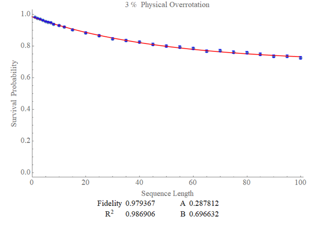
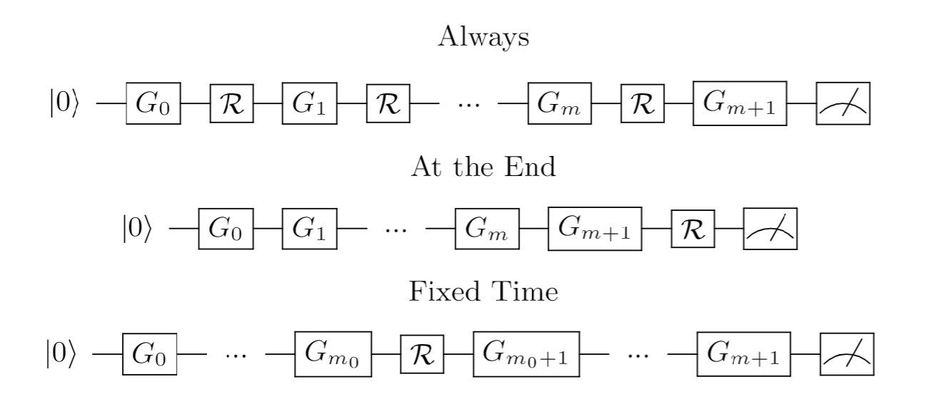
RB and LFE sequences sample noisy circuits whose output is known and measures the probability that the correct output is obtained, commonly known as the survival probability. A typical RB sequence is shown in the quantum circuit below where ...are selected randomly from the available gate set (usually the clifford group) and the gate = would invert every gate before it if the sequence were implemented perfectly. RB theory typically asserts that for an RB sequence without trace loss, the survival probability is an exponential decay in the sequence length [3, 6, 14, 26, 27, 28, 39, 59, 62]. The base of this exponential decay is the average fidelity, the figure of merit typically estimated with RB. We plot the survival probability for certain sequence lengths with blue dots surrounded by error bars and, when relevant, we show a red line representing an exponential fit to the data. Each blue dot represents the average outcome 100 RB sequences performed at the given sequence length unless otherwise stated. Parameters extracted from the exponential decay are listed below the plot. See the example plot below.The main distinction between RB and LFE is in LFE we use the stabilizer code at some point in the LFE sequence. We pick from 3 possibilities as a starting point to design LFE procedures:1. Always - Use the stabilizer code after every implemented gate.2. At the End - Use the stabilizer code at the end of the sequence.3. At Fixed Time - Use the stabilizer code at a fixed sequence length (in this notebook we use sequence length 50 exclusively).We enumerate the above options using the quantum circuits below, representing the action of the stabilizer code with the box labeled with script R.
G
1
G
m
G
m+1
†
()
m
∏
i=1
G
i

In addition to when we use stabilizer code, we also have freedom in the way we use stabilizer codes in the LFE gate sequence. We limit ourselves to 3 uses of the stabilizer code: QEC, Rejected Post-selection, and DIscarded post-selection.
1. QEC - uses the output of the stabilizer measurement to insert a Pauli meant to invert the error pattern associated with the measurement outcome.
2. Rejected post-selection - when an error is detected by the stabilizer measurement, the implemented sequence is treated as if a fatal error occurred in the implementation of the logical gates.
3. Discarded post-selection - when an error is detected by the stabilizer measurement, the implemented sequence is treated as if it did not happen.
Combining each of the choices given above gives 9 LFE procedures which we will investigate in depth. The merits of each will be explored in their respective subsections below.
All simulated data in this notebook is taken with physical filp noise in the X direction for each qubit see the Define Error Models chapter for details.
1. QEC - uses the output of the stabilizer measurement to insert a Pauli meant to invert the error pattern associated with the measurement outcome.
2. Rejected post-selection - when an error is detected by the stabilizer measurement, the implemented sequence is treated as if a fatal error occurred in the implementation of the logical gates.
3. Discarded post-selection - when an error is detected by the stabilizer measurement, the implemented sequence is treated as if it did not happen.
Combining each of the choices given above gives 9 LFE procedures which we will investigate in depth. The merits of each will be explored in their respective subsections below.
All simulated data in this notebook is taken with physical filp noise in the X direction for each qubit see the Define Error Models chapter for details.
Randomized Benchmarking with Logical Operators
Randomized Benchmarking with Logical Operators
First, we examine a standard RB procedure performed with logical gates and we do not make use of the stabilizer code to reduce errors. Currently, the most robust and thoroughly peer reviewed incarnation of RB is Character Benchmarking [28] so we will technically be making use of this framework during this notebook.
However, all the reader need know is that our procedure performs the RB sequence stated above with the Logical Asymmetric Group and that the Logical Asymmetric Group is sufficient for one to observe an exponential decay just as one would expect with the Clifford group on a single physical qubit. See chapters 7 and 3 of my thesis for a more thorough explanation as to why the Logical Asymmetric Group is a suitable group for Character Benchmarking.
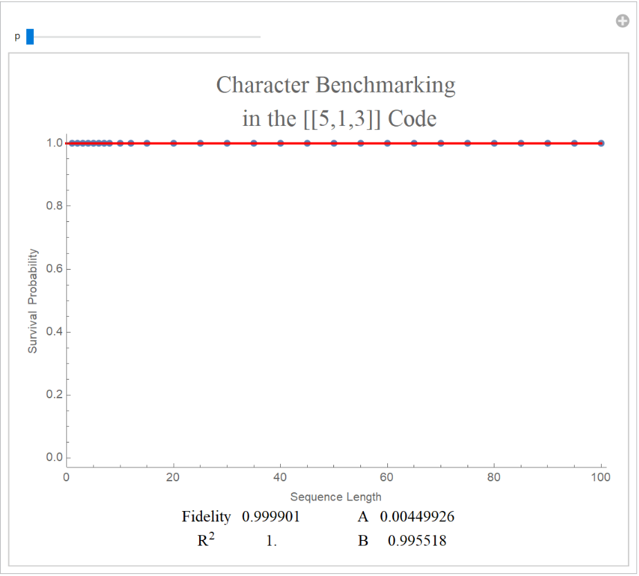
Now we look at our first data generated by this notebook. Manipulating the variable p in the cell below will use adjust the severity of the noise being considered. Specifically, we allow p to range from a 0% chance of error to a .6% chance of error.
Run the Cell below to display the data! A screenshot is shown of the output. Please download the notebook and evaluate the code to see the interactive object.
However, all the reader need know is that our procedure performs the RB sequence stated above with the Logical Asymmetric Group and that the Logical Asymmetric Group is sufficient for one to observe an exponential decay just as one would expect with the Clifford group on a single physical qubit. See chapters 7 and 3 of my thesis for a more thorough explanation as to why the Logical Asymmetric Group is a suitable group for Character Benchmarking.
Now we look at our first data generated by this notebook. Manipulating the variable p in the cell below will use adjust the severity of the noise being considered. Specifically, we allow p to range from a 0% chance of error to a .6% chance of error.
Run the Cell below to display the data! A screenshot is shown of the output. Please download the notebook and evaluate the code to see the interactive object.
In[]:=
SurvivalPlot["Character Benchmarking"]
Out[]=
Logical Fidelity Estimation with Quantum Error Correction
Logical Fidelity Estimation with Quantum Error Correction
QEC Always
QEC Always
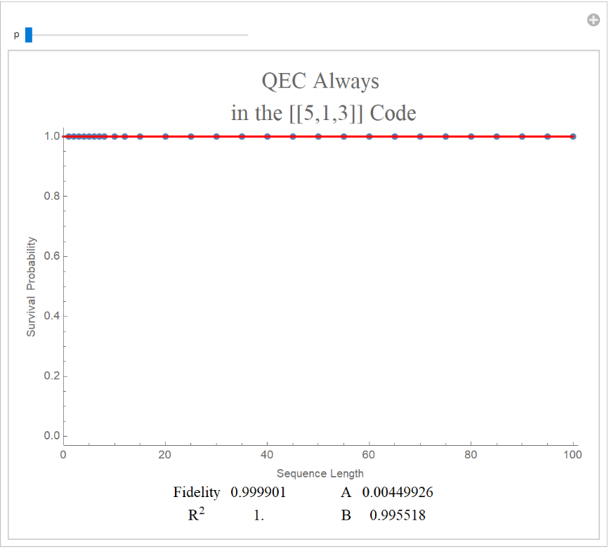
We perform QEC with the minimum weight decoder after every gate in the LFE sequence.
We first present data taken when QEC is performed with each logical gate, otherwise known as QEC Always LFE. Here we show that for physical overrotation noise, this resource intensive protocol gives monotonically decreasing results which roughly fit the typical exponential curve used in RB.This was expected for the gate-independent noise models that were used in this notebook, this was shown in Theorem 6.1 and Corollary 6.1 of my thesis.
The probability of applying an X gate independently to each qubit is controlled by p.
We first present data taken when QEC is performed with each logical gate, otherwise known as QEC Always LFE. Here we show that for physical overrotation noise, this resource intensive protocol gives monotonically decreasing results which roughly fit the typical exponential curve used in RB.This was expected for the gate-independent noise models that were used in this notebook, this was shown in Theorem 6.1 and Corollary 6.1 of my thesis.
The probability of applying an X gate independently to each qubit is controlled by p.
In[]:=
SurvivalPlot["QEC Always"]
Out[]=
QEC at the End
QEC at the End
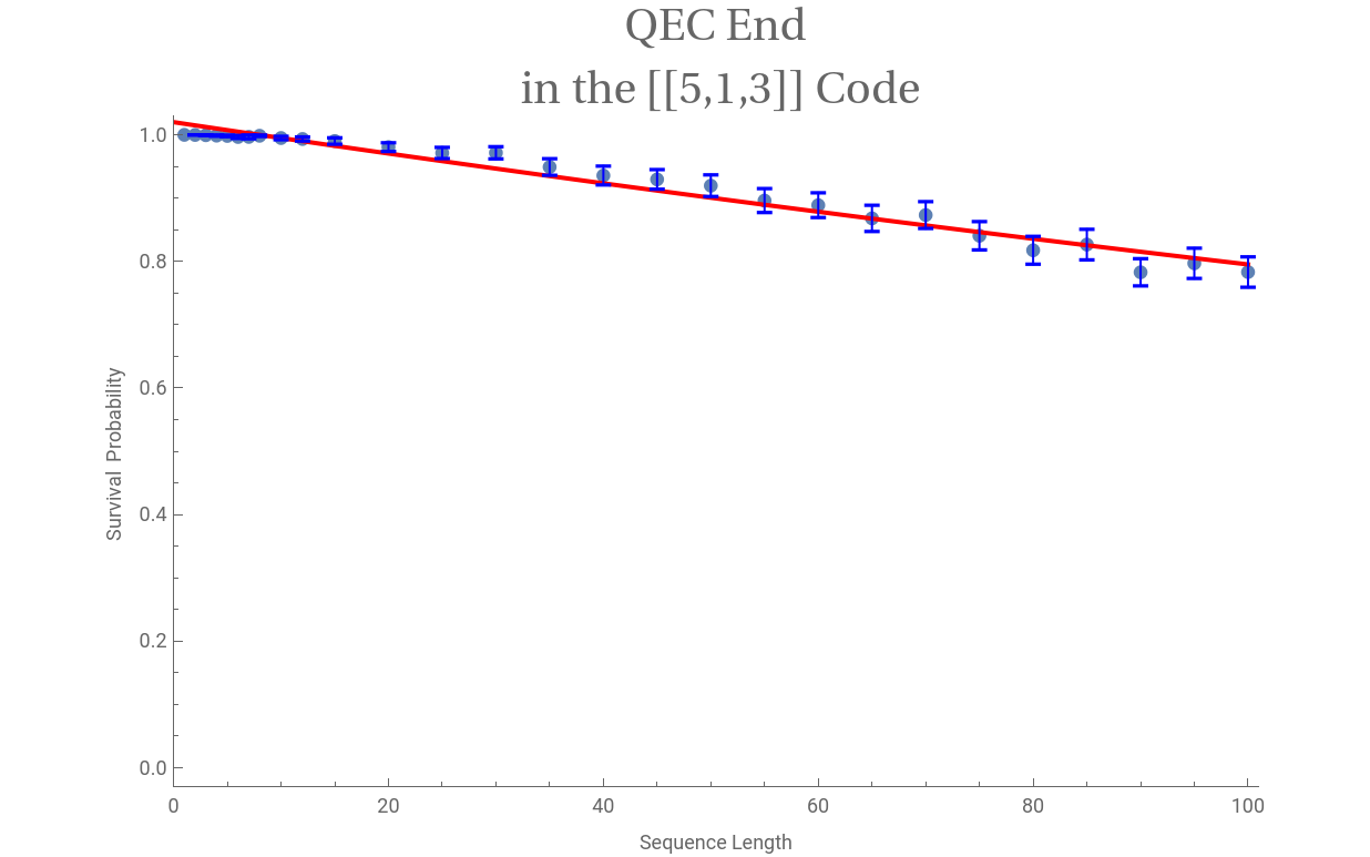
Now we only perform QEC after the final gate in the RB sequence. Again, the probability of applying an X gate independently to each qubit is controlled by p.
QEC at Fixed Time
QEC at Fixed Time
FInally, we present a procedure where QEC is applied after a fixed number of gates are performed. Namely, we perform QEC after 50 gates are performed in the LFE sequence. The exponential fit model is omitted from this plot as there is no reason to suspect that the decay should follow an exponential.
Again, the probability of applying an X gate independently to each qubit is controlled by p. This plot shows the error threshold the most clearly, as for the first few values of p the survival rate is almost completely restored. However, one sees a quick drop in effectiveness of QEC once errors are above the threshold.
Again, the probability of applying an X gate independently to each qubit is controlled by p. This plot shows the error threshold the most clearly, as for the first few values of p the survival rate is almost completely restored. However, one sees a quick drop in effectiveness of QEC once errors are above the threshold.
Logical Fidelity Estimation with Post Selection
Logical Fidelity Estimation with Post Selection
LFE experiments using post-selection can be done in post-processing using the syndromes obtained from performing QEC.
Define Error Models
Choose which error models are being used by re-defining UpdateErrorFunctions.
Default choices for error models are chosen based on which overrotations are interesting.
One can write any Pauli using σ=LST so finding the Pauli over rotations which are interesting. Let’s examine the combinations, ignoring those which include stabilizers as stabilizers have no overall affect on the syndrome measurement outcome.
Just logical overrotations is equivalent to errors on a single qubit in physical RB.
All that’s left to explore is the destabilzier overrotations and the Paulis which are made from destabilizers and logical, both of which we explore in earnest.
One can write any Pauli using σ=LST so finding the Pauli over rotations which are interesting. Let’s examine the combinations, ignoring those which include stabilizers as stabilizers have no overall affect on the syndrome measurement outcome.
Just logical overrotations is equivalent to errors on a single qubit in physical RB.
All that’s left to explore is the destabilzier overrotations and the Paulis which are made from destabilizers and logical, both of which we explore in earnest.
We require that the error is parameterized by the independent variables p and θ. Generally, p controls the probability of an error and θ controls degree of overrotation.
Define which Error values we wish to test.
Logical Fidelity Estimation
Runs character Benchmarking by default. Unless a QEC modifier is specified, it is assumed that the interleaved R is QEC. To do post-selection, one must pick a QEC modifier below.
Any procedure that uses a tag from the first line should produce accurate results.
Any procedure that uses a tag from the first line should produce accurate results.
Save, Display, and Retrieve Data
Survival Probability Plot
Survival Probability Plot
Error Bars may be a little bit wonky for low sample sizes. A screenshot is shown of the output. Please download the notebook and evaluate the code to see the interactive object.
Save and Manipulate Data
Save and Manipulate Data
I save data in .mx files in 3 associations {DataBase,DataInfo,FitModels} as you can see below.
DataBase shows raw physical data for each procedure
DataInfo gives various specs on the RB run including error model description, gate set used, sequence lengths tested, etc...
FitModels is an association of NonLinearModelFit Objects for each of the benchmarks in DataBase https://reference.wolfram.com/language/ref/NonlinearModelFit.html
DataBase shows raw physical data for each procedure
DataInfo gives various specs on the RB run including error model description, gate set used, sequence lengths tested, etc...
FitModels is an association of NonLinearModelFit Objects for each of the benchmarks in DataBase https://reference.wolfram.com/language/ref/NonlinearModelFit.html