Nestedly recursive functions are functions that have to call themselves (recursion), multiple times (nesting). Complex patterns emerge from these seemingly simple but nested functional forms. This project first implements a stack-based recursive function from scratch to have more introspection into how the recursion works. Then, it explores the function space of various kind of shift operators. The call graphs of these relatively basic shifting operations exhibit interesting, complex and sometimes fractal patterns. We also explore simple arithmetic operations, although that function space is more limited. We find patterns that are tree and branch-like as well as flowers and even a type of marine coral.
Introduction & Definitions
Introduction & Definitions
A. Nestedly recursive functions
A. Nestedly recursive functions
A recursive function is a function for which its result depends on a previous result of the same function. We say that recursive functions “call themselves”. These functions do so until certain initial conditions are met. Probably the most famous recursive function is the Fibonacci sequence: . Where the initial conditions are
F(n) = F(n - 1) + F(n - 2)
F(0) = 0 and F(1) = 1
In[]:=
recursivefibonacci=NestedRecursiveFunction[F[n]F[n-1]+F[n-2],{},{n00,n11}];stackfibonacci=NestedRecursiveFunctionWhile[F[n]F[n-1]+F[n-2],{},{n00,n11}];
Nestedly recursive functions are recursive functions that call themselves multiple times, in a nested fashion. This was termed by Stephen Wolfram, and an example is Hofstadter’s Q-Sequence:
Q(n) = Q(n - Q(n - 1))+Q(n - Q(n - 2))
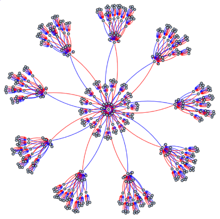
The call graph of a nestedly recursive function show us the the previous results of the function that were used to compute the current result. For example, for the Fibonacci sequence:
In[]:=
recursivefibonaccigraph=CallGraph[FunctionCallGraph[recursivefibonacci,10]]
Out[]=
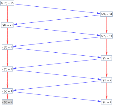
The color of the edges represent the order of the calls. Red is the first call, blue is the second, green is the third and yellow is the fourth. The number of times a function calls itself is thus depicted by the colors of the edges.
B. Emergence of complexity
B. Emergence of complexity
“All the wonders of our universe can in effect be captured by simple rules, yet ... there can be no way to know all the consequences of these rules, except in effect just to watch and see how they unfold.” Stephen Wolfram
We are using this simple concept from Stephen Wolfram and applying it to a specific mathematical structure. The hypothesis is that complexity emerges from simple recursive functional forms, and even more so from nestedly recursive functional forms. Instead of looking at just the two previous numbers as in the Fibonacci sequence, we look at multiple previous results, with varying distances from the current input. This complexity can be visualised with call graphs, where we might see interesting patterns. Stephen Wolfram has already looked at the graphs of some of these forms, and this initial exploration is the basis for this project. Below are some of the functional forms and graphs that Stephen Wolfram has already explore, we are visualising those below:
For example, the following form from OEIS-A002024 and NKS page 129a, gets us a cone-shaped structure:
F(n) = 1 + F(n - F(n - 1)),
In[]:=
CallGraphNoLabels[FunctionCallGraph[NestedRecursiveFunction[F[n]1+F[n-F[n-1]],{},{n≤11}],300]]
Out[]=
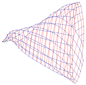
OEIS-A046699, from NKS page 129d, ), gets us a pattern that resembles an ammonite:
F(n) = F(n-F(n-1)) + F(n - F(n - 2) - 1)
In[]:=
CallGraphNoLabels[FunctionCallGraph[NestedRecursiveFunction[F[n]F[n-F[n-1]]+F[n-F[n-2]-1],{},{n≤21}],300]]
Out[]=

We see that this function calls itself four times, meaning we get vertices with the yellow color, representing the fourth call of the function.
Programming Nestedly Recursive Functions
Programming Nestedly Recursive Functions
Mathematica allows us to define recursive functions out of the box, as such, for the Fibonacci sequence:
In[]:=
fib[0]=0;fib[1]=1;fib[n_]:=fib[n]=Plus[fib[n-1],fib[n-2]]fib[10]
Out[]=
55
However, this simple function encounters problems when the recursion is very large. It will hit a recursion depth limit.
In[]:=
fib[10^4]

Out[]=
2TerminatedEvaluation[RecursionLimit]
It is possible to manually increase the recursion depth limit to avoid this error. Nevertheless, it would be ideal to create a function that does not encounter this issue from the start. Therefore, the first part of the project was to implement a function that could deal with nested recursive functions. This function should have the following characteristics:
◼
memoization: it should remember results it has computed previously and avoid recomputing them. This is especially important if we want to compute results for a range of numbers.
◼
avoiding recursion depth limit errors
◼
accepting functional forms: all kinds of complex forms should be dealt with in a flexible and smooth manner.
A. Memoized recursive function
A. Memoized recursive function
The first iteration of this function is named NestedRecursiveFunction and was implemented by Brad Klee, with help from Stephen Wolfram. It can be found at the bottom of this notebook in the Code section. This version is fast, accepts complex functional forms and uses memoization. It also outputs the edges needed to create those call graphs with the FunctionCallGraph, CallGraph and CallGraphNoLabels functions.
B. Stack-based recursive function
B. Stack-based recursive function
The second iteration is named NestedRecursiveFunctionWhile and can also be used to visualise the call graphs in the same way.
The difference here is that the function does not call itself. We implement the call stack ourselves and traverse the call graph up and down. The advantage is that we have more introspection into what is happening in the function, can estimate the computational complexity, and can optimise the memory storage and allocation. The disadvantage is that the first version of this function, which calls itself is much faster, probably due to some internal optimisation made by Mathematica. We should note that Mathematica probably also uses a stack-based method to compute functions that call themselves.
The difference here is that the function does not call itself. We implement the call stack ourselves and traverse the call graph up and down. The advantage is that we have more introspection into what is happening in the function, can estimate the computational complexity, and can optimise the memory storage and allocation. The disadvantage is that the first version of this function, which calls itself is much faster, probably due to some internal optimisation made by Mathematica. We should note that Mathematica probably also uses a stack-based method to compute functions that call themselves.
C. Runtime comparisons
C. Runtime comparisons
Below are the runtime statistics of these three implementations of a recursive function.
In[]:=
data={{n,simple,recursive,"stack based"},{10,RepeatedTiming[fib[10]][[1]],RepeatedTiming[recursivefibonacci[10]][[1]],RepeatedTiming[stackfibonacci[10]][[1]]},{10^2,RepeatedTiming[fib[10^2]][[1]],RepeatedTiming[recursivefibonacci[10^2]][[1]],RepeatedTiming[stackfibonacci[10^2]][[1]]},{10^3,RepeatedTiming[fib[10^3]][[1]],RepeatedTiming[recursivefibonacci[10^3]][[1]],RepeatedTiming[stackfibonacci[10]^3][[1]]},{10^4,RecursionLimit,RepeatedTiming[recursivefibonacci[10^4]][[1]],RepeatedTiming[stackfibonacci[10^4]][[1]]}};
Note that for this simple Fibonacci sequence, the stack-based implementation performs better, but for more complex functional forms, the result is more ambiguous.
D. Testing
D. Testing
The most important aspect of our implementations is that they do not hit recursion depths, unlike the simple one we saw first. We can check this with the Fibonacci sequence of 10’000.
And the results match:
Then, we want to test that the call graphs are the same for both functions.
Shift-based Operations
Shift-based Operations
These shift operations are found everywhere in recursive functions. Here, we want to come up with some relatively simple shift operators that could be used in our nestedly recursive functions to create some interesting patterns in their call graphs. Shifters are complex in themselves, so we expect some complex patterns to emerge from them. Note that these operators must decrease the initial integer, so that the recursive function reaches an initial condition and stops. This will avoid the unbounded growth problem we mentioned above. Below is an explanation of these shifters and some functional forms that gave us interesting patterns. A lot of the following shift methods have been devised by Brad Klee. Most of the methods that we will be using in this section will convert a number into its decimal digits, apply some kind of transformation to these digits, and then convert them back into an integer. The base will usually be defined by the user.
A. Chop Shift
A. Chop Shift
Chop Shift converts the input integer into its decimal digits. Then the user defines either Most or Rest and takes the first elements except the last one (Most) or all the elements except the first (Rest) and converts these numbers back into an integer. Since we are always left with a digit less than the input digits, the output integer will always be smaller than the input one.
Here Chop Shift is introduced in a recursive function with base 2.
The following line plot for this functional form gives us an interesting pattern that repeats itself, but still follows an upward trajectory.
Here, we see some distinct communities, where many nodes are clustered together, with just a few nodes acting as bridges between values.
Adding two Chop Shift operators with very different bases, as above, gives us this shape, with one central node having an outsized importance.
Again, a specific combination of bases can give us some relatively beautiful looking shapes.
B. Cellular Automaton Shift
B. Cellular Automaton Shift
Cellular Automaton Shift transforms the decimal digits of the input integer based on a specific Cellular Automaton (CA) rule. We then take all elements except the last one (Rest) to make sure our output integer is smaller. The CA rule is set by the user. Since CA rules only deal with binary numbers (0 and 1), we set the base to 2 for this shifter.
The graphs from the CA Shift are very dependent on the rule set by the user. The current function just chooses two random rules for this recursive function.
C. Flip Shift
C. Flip Shift
Flip Shift converts each decimal digit, n, to their previous number, n-1. Note that no decimal digit sequence can start with 0 and a 0 will be converted to a 1.
The line plot for Flip Shift gives us an interesting pattern, that looks like small spaceships. The call graphs are, however, not very interesting.
D. Expand Shift
D. Expand Shift
Expand Shift gives a list of the decimal digits of the input integer multiplied by their corresponding powers of 10. We then take the Rest of these digits and total them.
Again, the line plot has a more interesting pattern than the call graphs for Expand Shift.
E. Digit Shift
E. Digit Shift
Digit Shift simply takes the sum of all the digits of the input integer.
The line plot outputs clearly defined lozenge, of the same size, separated from each other, but following an upward trend.
Interestingly, Digit Shift gives us disconnected graphs, where most of them have a very central node, that acts as the center of the graph.
A similar pattern, here. Even with more nodes we get a few very small subgraphs next to other, very dense, subgraphs.
F. Split Shift
F. Split Shift
Split Shift simply chops off the first element of the input integer. 157 will become 57, 57 will become 7, and so on.
We seem to have almost identically looking subgraphs next to each other.
This simple nested recursive function gives us a circular shape, that is very dense.
I. Extra - Dragon
I. Extra - Dragon
The following methods are either taken directly from Brad Klee’s blog post on A new dragon theorem or were inspired by it. Brad explored a paper folding dragon curve in this blog post. See Brad’s post for a more in depth explanation of Clumsy Shift and Cycle Shift.
1. Clumsy Shift
1. Clumsy Shift
Clumsy Shift gives us a branch-like structure, where subtrees grow out from other subtrees.
2. Cycle Shift
2. Cycle Shift
Cycle Shift also gives us a branch-like structure.
3. Split Chop Shift Length
3. Split Chop Shift Length
Split Chop Shift Length takes the length of the decimal digits of the input integer.
Here, we have very dense communities that are linked to each other by only one edge.
This slightly different function also gives us dense communities that are still connected to each other.
4. Split Chop Shift
4. Split Chop Shift
Split Chop Shift does a similar operation but converts the resulting list into an integer, instead of taking its length.
Split Chop Shift outputs a shape that looks like a flower, and the patterns look the same for each individual branch, making it symmetrical.
Basic Arithmetic Operations
Basic Arithmetic Operations
The most basic arithmetic operations have already been explored by Stephen Wolfram in his book, A New Kind of Science. Here we look to explore similar functions with different parameters or tweak them with different basic arithmetic operations. We systemized the creation of these functional forms, to better explore the function space. Below are a select few that created interesting patterns.
A. Addition, Subtraction & Multiplication
A. Addition, Subtraction & Multiplication
Here we used the initial functional forms from Stephen Wolfram with different parameters. Not all of these are fully nested, some are just recursive.
With a larger input, we get a more and more dense tube-like structure.
Similarly, we get a slightly wider tube-like pattern again.
Now, we also get a tube-like structure, but two, disconnected ones.
B. Square Root
B. Square Root
The patterns using square roots, do not give us very interesting patterns, except for this one, using the Floor operator.
C. Division Operations: Divide, Floor, Ceiling, Modulo & Quotient
C. Division Operations: Divide, Floor, Ceiling, Modulo & Quotient
In general, we found some patterns when using division operations in conjunction with Floor and Ceiling, to get whole integers.
This looks like an incomplete wheel, with a node sticking out and preventing it from closing the wheel.
Finally, we have a a pattern that looks like a coral, which are marine invertebrates. This pattern specifically resembles a lettuce coral.
Future Direction
Future Direction
Our stack-based recursive function can possibly be optimised in multiple ways. First, we can set a condition to prevent unbounded growth, and thus, avoid the function running forever. Second, we could further optimise memory storage by not recomputing the partials that are shared across functions. Partials are the parts of the function that are calculated separately in the function to get the final result. Ideally, our implementation would be just as performant as the recursive method. However, with the optimisation that is done in the background by Mathematica, it is unlikely we would reach this state at this level of abstraction.
Regarding the function space, there are countless combinations of arithmetic operations and functional forms to test. We have just shown the few of our many experiments that created interesting patterns. Of course, we haven’t tested all possibilities. However, one limit is the size of the graph. One can increase the size of the input integer to a very large number, but the visualisation of these call graphs will not be as useful to look at, if they can even rendered at all.
Regarding the function space, there are countless combinations of arithmetic operations and functional forms to test. We have just shown the few of our many experiments that created interesting patterns. Of course, we haven’t tested all possibilities. However, one limit is the size of the graph. One can increase the size of the input integer to a very large number, but the visualisation of these call graphs will not be as useful to look at, if they can even rendered at all.
Conclusion
Conclusion
This project has looked at different ways to implement nestedly recursive functions. Our novel, stack-based approach deals with an arbitrarily deep recursion.
We’ve also explored various shift operators. Most of them convert an integer into decimal digits, apply a transformation and then convert it back to an integer. These shifters do manage to create complex patterns in their call graphs.
Using simple arithmetic operations is indeed limited and was already explored by Stephen Wolfram in the past. We extended this exploration by systemizing the analysis of these functional forms by playing around with their parameters, and did find complex call graphs. However, there often seems to be a trade-off between the complexity of the functional form and the attractiveness of the call graphs it outputs.
As Stephen Wolfram said “there’s a possibility of a more general basis for rules to describe nature”. The hypothesis that relatively simple functional forms can create complex patterns is validated. We found patterns that are present in the natural world, patterns that resemble organisms as complex as branches, flowers and corals.
Keywords
Keywords
◼
Recursive functions
◼
Memoization
◼
Call Graphs
◼
Shifters
Acknowledgments
Acknowledgments
I would like to sincerely thank Brad Klee for his guidance, teaching and patience. Brad was an incredible mentor and provided me with invaluable code snippets, ideas and support. He also fostered a great team and I want to thank Maria Fernanda Castro, Zsombor Méder, Atik Santellán and Jakub Trzaska for making this summer school memorable. Lastly, I’d like to thank Stephen Wolfram for enabling me to explore these fascinating topics and creating this great community of Wolfram thinkers and innovators.
References
References
1
.Stephen Wolfram (2002), p128-129-130 & notes 4-3, “A New Kind of Science”. https://www.wolframscience.com/nks/
2
.Stephen Wolfram (2011), “Call Graphs of Nestedly Recursive Functions”. http://demonstrations.wolfram.com/CallGraphsOfNestedlyRecursiveFunctions/
3
.Stephen Wolfram (2011), “Multiterm Nestedly Recursive Functions”. http://demonstrations.wolfram.com/MultitermNestedlyRecursiveFunctions/
4
.Stephen Wolfram (2011), “One-Term Nestedly Recursive Functions”. http://demonstrations.wolfram.com/OneTermNestedlyRecursiveFunctions/
5
.Enrique Zeleny (2011), “Tree Form of Recursive Function Evaluation Steps”. http://demonstrations.wolfram.com/TreeFormOfRecursiveFunctionEvaluationSteps/
6
.Bradley Klee (2024), “A new dragon theorem”. https://community.wolfram.com/groups/-/m/t/3208738
Cite This Notebook
Cite This Notebook