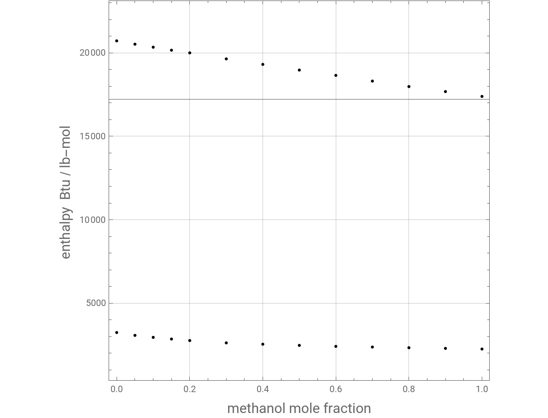
We plot of the Ponchon-Savarit diagram (i.e., (y) and (x)) for a methanol-water mixture at a total pressure, P=760 mmHg.
In addition, the tie lines or isotherms are shown in green.
The data obtained in our simulation agrees very well with those given in Henley and Seader’s classic textbook [1], which are
given below and shown by red dots in the diagram.
Finally, we depict the vapor-liquid equilibrium data in a separate diagram.
Reference:
[1] E. J. Henley and J. D. Seader, Equilibrium-Stage Separation Operations in Chemical Engineering, New York: Wiley, 1981.
Expressions for pure component vapor and liquid enthalpies were adapted from Aspen-HYSYS. Enthalpies are above and are given in .
H
v
h
l
In addition, the tie lines or isotherms are shown in green.
The data obtained in our simulation agrees very well with those given in Henley and Seader’s classic textbook [1], which are
given below and shown by red dots in the diagram.
Finally, we depict the vapor-liquid equilibrium data in a separate diagram.
Reference:
[1] E. J. Henley and J. D. Seader, Equilibrium-Stage Separation Operations in Chemical Engineering, New York: Wiley, 1981.
Expressions for pure component vapor and liquid enthalpies were adapted from Aspen-HYSYS. Enthalpies are above
0°C
Btu/lb-mol
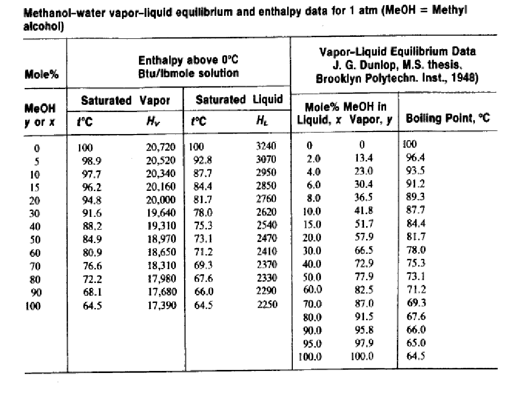
Plot of the data provided in Henley and Seader' s textbook (i.e., enthalpies expressed in Btu/lbmol)
In[]:=
P1=Show[ListPlot[{{0,20720},{0.05,20520},{0.1,20340},{0.15,20160},{0.2,20000},{0.3,19640},{0.4,19310},{0.5,18970},{0.6,18650},{0.7,18310},{0.8,17980},{0.9,17680},{1.0,17390}},PlotStyle{Red,PointSize[0.022]},FrameTrue,FrameLabel{Style["methanol mole fraction",14],Style["enthalpy Btu / lb-mol ",14]},GridLinesAutomatic,ImageSize{550,420},PlotStyleThick,AspectRatio1],ListPlot[{{0,3240},{0.05,3070},{0.1,2950},{0.15,2850},{0.2,2760},{0.3,2620},{0.4,2540},{0.5,2470},{0.6,2410},{0.7,2370},{0.8,2330},{0.9,2290},{1.0,2250}},PlotStyle{Red,PointSize[0.022]},FrameTrue,FrameLabel{Style["methanol mole fraction",14],Style["enthalpy Btu / lb-mol ",14]},GridLinesAutomatic,ImageSize{550,420},PlotStyleThick,AspectRatio1],PlotRange{{0,1},{1500,22000}}]
Out[]=
Total pressure is set equal to 760 mmHg
In[]:=
P=760
Out[]=
760
Antoine Constants and equation for methanol and water.
In[]:=
Aa1=8.08097;Ba1=1582.271;Ca1=239.726;Aa2=8.07131;Ba2=1730.63;Ca2=233.426;Psat1=10^(Aa1-Ba1/(T+Ca1));Psat2=10^(Aa2-Ba2/(T+Ca2));
Binary interaction parameters for the Van Laar activity coefficient model
In[]:=
A12=0.76429;A21=0.62569;Gam1[xa_]:=Exp[A12(A21(1-xa)/(A12xa+A21(1-xa)))^2];Gam2[xa_]:=Exp[A21(A12xa/(A21(1-xa)+A12xa))^2];
Computing VLE data for the binary system: methanol and Water
In[]:=
i=0;While[i<1001,{xa=i0.001,sol=FindRoot[Psat1xaGam1[xa]+Psat2(1-xa)Gam2[xa]P,{T,77,78}];xe[i]=xa,ye[i]=Psat1xaGam1[xa]/P/.sol,Te[i]=T/.sol,i++}];Tbl1=Table[{xe[i],Te[i]},{i,0,1000}];Tbl2=Table[{ye[i],Te[i]},{i,0,1000}];Tbl3=Table[{xe[i],ye[i]},{i,0,1000}];Tx=Interpolation[Tbl1,InterpolationOrder1];Ty=Interpolation[Tbl2,InterpolationOrder1];xy=Interpolation[Tbl3,InterpolationOrder1];
vapor-phase and liquid-phase enthalpies of the mixture (expressed in Btu/lbmol)
In[]:=
A=(0.0+105.80T-0.181115100T^2+3.1263370010^-004T^3-3.6393090010^-013T^4)/.T(273.15);hl1=0.0+105.80T-0.181115100T^2+3.1263370010^-004T^3-3.6393090010^-013T^4-A;B=(0.0+76.2820400T+2.5651420010^-002T^2-1.1279380010^-004T^3+1.3259630010^-007T^4)/.T(273.15);hl2=0.0+76.2820400T+2.5651420010^-002T^2-1.1279380010^-004T^3+1.3259630010^-007T^4-B;Hv1=50918.3600+93.976T-0.374347200T^2+7.9373420010^-004T^3-6.269264010^-007T^4-A;Hv2=47304.1700+107.579100T-0.220258100T^2+3.6616110010^-004T^3-3.2280850010^-007T^4-B;Hvhysys[y_]:=0.94782×0.45359237(yHv1+(1-y)Hv2)/.T(Ty[y]+273.15);hlhysys[x_]:=0.94782×0.45359237(xhl1+(1-x)hl2)/.T(Tx[x]+273.15);
Plot of the Ponchon-Savarit diagram at P=760 mmHg.
Tie-lines are given in Green.
Dew line and bubble line are in Yellow and Blue.
Tie-lines are given in Green.
Dew line and bubble line are in Yellow and Blue.
In[]:=
P2=Show[Plot[{hlhysys[x],Hvhysys[x]},{x,0,1},FrameTrue,FrameLabel{Style["methanol mole fraction",14],Style["enthalpy Btu / lb-mol ",14]},GridLinesAutomatic,ImageSize{550,420},PlotStyleThick,PlotRange{{0,1},All},AspectRatio1],Graphics[{Thick,Green,Table[Line[{{i,hlhysys[i]},{xy[i],Hvhysys[xy[i]]}}],{i,0,1,.05}],Black,Table[Style[Text[Row[{ToString[NumberForm[Tx[i],{4,2}]]," °C"}],{(i+xy[i])/2+0.001,(hlhysys[i]+Hvhysys[xy[i]])/2},Automatic,{10000,(hlhysys[i]-Hvhysys[xy[i]])/(i-xy[i])+10}],10],{i,0.05,0.95,0.05}]}]]
Out[]=
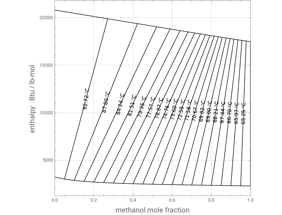
Comparison of our data with their counterparts (the red dots) reported in Henley and Seader’s textbook (Ref. 1).
In[]:=
Show[P1,Show[Plot[{hlhysys[x],Hvhysys[x]},{x,0,1},FrameTrue,FrameLabel{Style["methanol mole fraction",14],Style["enthalpy Btu / lb-mol ",14]},GridLinesAutomatic,ImageSize{550,420},PlotStyleThick,PlotRange{{0,1},All},AspectRatio1]],AxesOrigin{0,1500}]
Out[]=
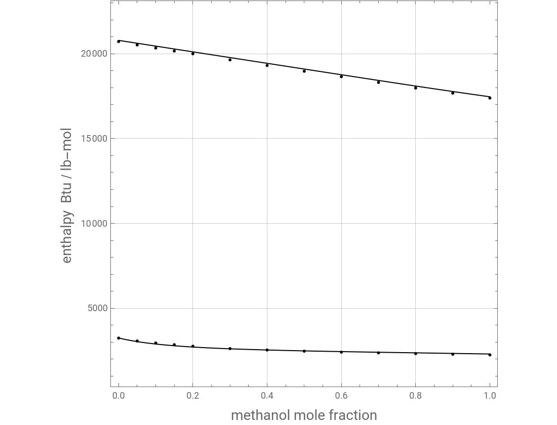
Plot of the VLE diagram at P=760 mmHg. Check of our VLE data against the values given in Ref. 1 (red dots)
CITE THIS NOTEBOOK
CITE THIS NOTEBOOK
Ponchon-Savarit Diagram for the Methanol-Water Binary Mixture at Atmospheric Pressure
by Housam Binous and Ahmed Bellagi
Wolfram Community, STAFF PICKS, January 12, 2024
https://community.wolfram.com/groups/-/m/t/3101318
by Housam Binous and Ahmed Bellagi
Wolfram Community, STAFF PICKS, January 12, 2024
https://community.wolfram.com/groups/-/m/t/3101318