What is LIDAR?
What is LIDAR?
LIght Detection And Ranging (LIDAR) makes use of a laser to excite backscattering in the atmosphere. This backscattered signal is observed using a telescope receiver. The optical signals received by the telescope are converted into electrical signals that are recorded and stored onto a computer.
Some Properties
Some Properties
- Range of wavelengths 250 nm - 11 um
- Laser source from different materials (solid state, gas)
- Laser source from different materials (solid state, gas)
Advantages of the LIDAR technique
Advantages of the LIDAR technique
- Continuous measurements of the vertical distribution of atmospheric components
- Increased spatial and temporal resolution
- Non destructive technique
- Increased range of measurements (50 m – 120 km)
- Simultaneous measurements of several constituents/pollutants
- Determination of air pollution sources
- Increased spatial and temporal resolution
- Non destructive technique
- Increased range of measurements (50 m – 120 km)
- Simultaneous measurements of several constituents/pollutants
- Determination of air pollution sources
The Calipso Lidar
The Calipso Lidar
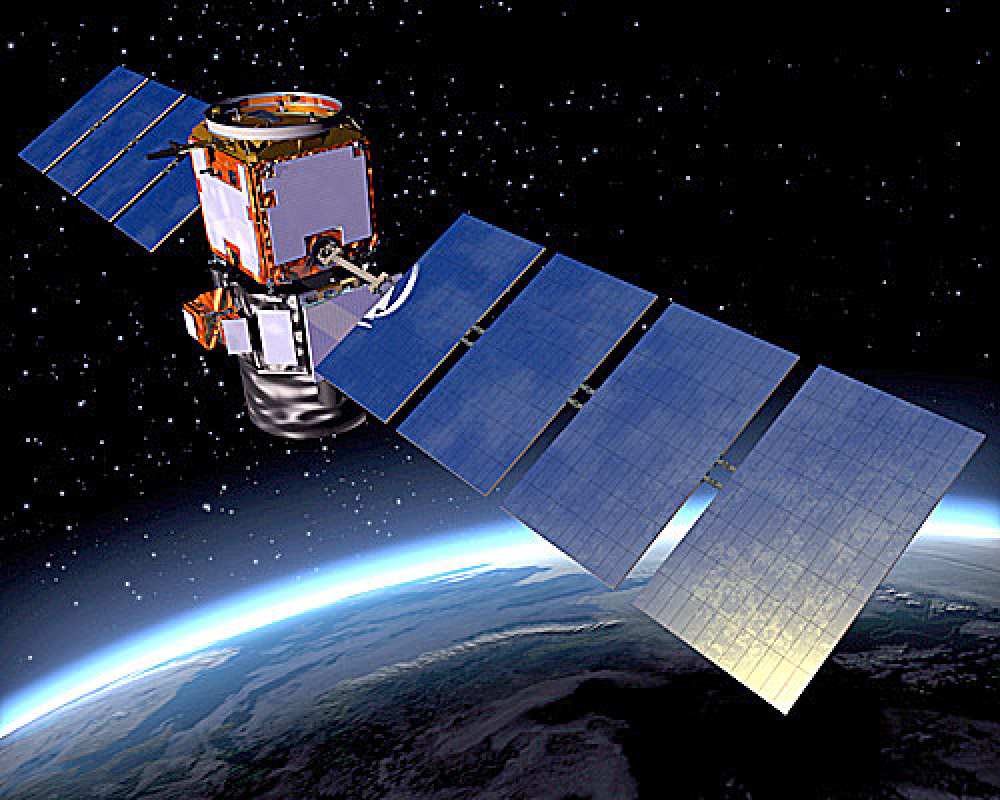
CALIPSO (Cloud-Aerosol Lidar and Infrared Pathfinder Satellite Observations) is a cloud and aerosol observation satellite operated by the National Aeronautics and Space Administration (NASA) and Centre National d’Etudes Spatiales (CNES). Its observations are used to determine the role of clouds and aerosols in regulating the Earth’s climate.CALIPSO carries three instruments: a Cloud-Aerosol Lidar with Orthogonal Polarisation (CALIOP), an Imaging Infrared Radiometer (IIR), and a Wide Field Camera (WFC). CALIOP uses a two-wavelength laser transmitter to obtain vertical profiles of clouds and aerosols from the detected backscatter. IIR provides context to nighttime CALIOP observations and acquires the size of particles within semi-transparent clouds, while WFC provides context for daytime CALIOP observations.
Retrieving Light Extinction (Attenuation) Data From the Calipso Satellite
Retrieving Light Extinction (Attenuation) Data From the Calipso Satellite
1. Loading Lidar DataFile
1. Loading Lidar DataFile
2. Extinction Coefficient (Light Attenuation Parameter)
2. Extinction Coefficient (Light Attenuation Parameter)
In[]:=
ArrayPlot[Reverse@Transpose[extinctionC],ColorFunction->(ColorData["TemperatureMap"][2*Clip[#,{0.,0.5}]]&),ColorFunctionScaling->False,PlotLegends->Placed[BarLegend[{(ColorData["TemperatureMap"][2*Clip[#,{0.,0.5}]]&),{0,0.5}}],Bottom],PlotLabel->"Extinction Coefficient (km^(-1))",ImageSize->Large,Axes->True,Ticks->{Table[{n,Column[coords[[n]]]},{n,Append[Range[1,4160,416],4160]}],Table[{n,altstrings[[n]]},{n,Append[Range[1,399,133],399]}]},Frame->False]
Out[]=


3. Ozone Number Density
3. Ozone Number Density
In[]:=
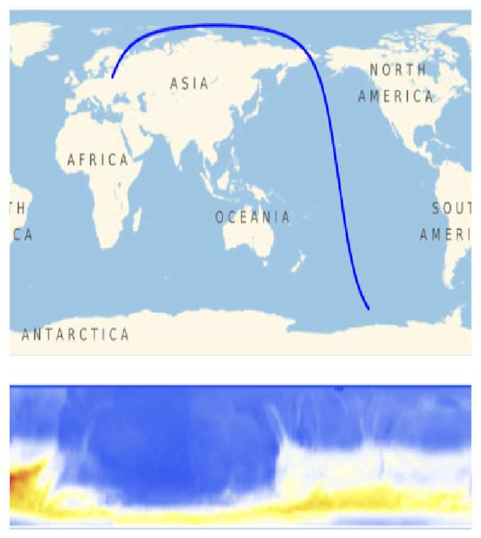
With[{end=4160},Module[{poly1,poly2,texture1,texture2},poly1=Polygon[{{0,0},{4,0},{4,3},{0,3}},VertexTextureCoordinates->{{0,0},{1,0},{1,1},{0,1}}];poly2=Polygon[{{0,-1.5},{4*N[end/4160],-1.5},{4*N[end/4160],-0.25},{0,-0.25}},VertexTextureCoordinates->{{0,0},{1,0},{1,1},{0,1}}];texture1=Rasterize[GeoGraphics[{LightRed,GeoPath[coords[[end;;]]],Blue,Thick,GeoPath[coords[[1;;end]]]}]];texture2=Rasterize[ArrayPlot[Reverse@Transpose@Take[ozone,end],ColorFunction->"TemperatureMap",Frame->False,PlotRangePadding->None]];Rasterize@Graphics[{Texture[texture1],poly1,Texture[texture2],poly2}]]]
Out[]=
In[]:=
Divisors[4160]
Out[]=
{1,2,4,5,8,10,13,16,20,26,32,40,52,64,65,80,104,130,160,208,260,320,416,520,832,1040,2080,4160}
3. Calipso Path Tracking and Ozone Detection
3. Calipso Path Tracking and Ozone Detection
In[]:=
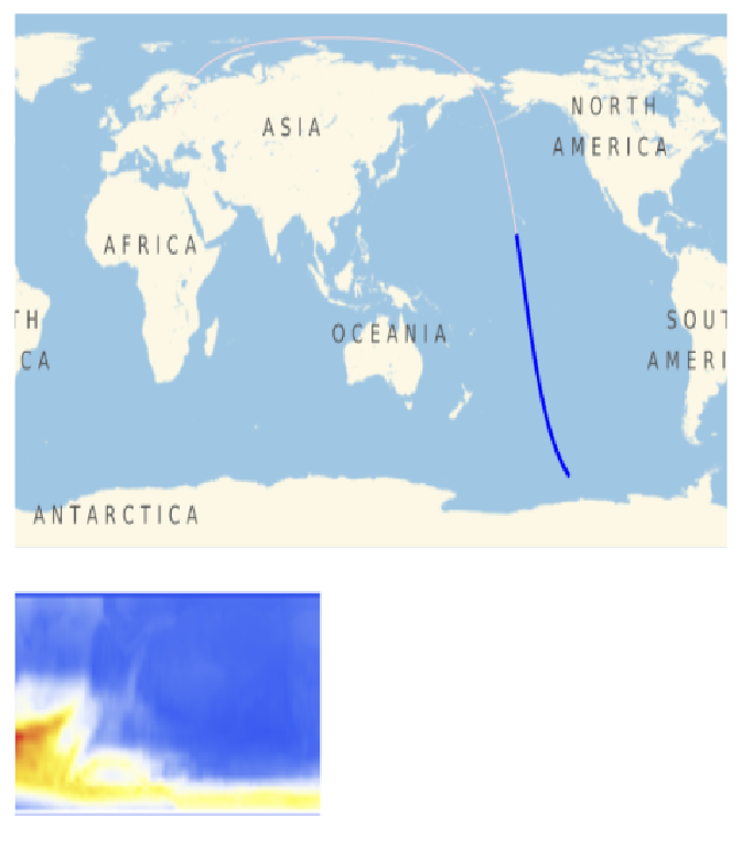
O3Video=Monitor[ListAnimate[With[{poly1=Polygon[{{0,0},{4,0},{4,3},{0,3}},VertexTextureCoordinates->{{0,0},{1,0},{1,1},{0,1}}],poly2=Polygon[{{0,-1.5},{4,-1.5},{4,-0.25},{0,-0.25}},VertexTextureCoordinates->{{0,0},{1,0},{1,1},{0,1}}],texture2=Rasterize[ArrayPlot[Reverse@Transpose@ozone,ColorFunction->"TemperatureMap",Frame->False,PlotRangePadding->None]]},Table[Module[{texture1,maskpoly},texture1=Rasterize[GeoGraphics[{LightRed,GeoPath[coords[[end;;]]],Blue,Thick,GeoPath[coords[[1;;end]]]}]];maskpoly=Polygon[{{4(N[end/4160]),-1.6},{4,-1.6},{4,-0.15},{4(N[end/4160]),-0.15}},VertexTextureCoordinates->{{0,0},{1,0},{1,1},{0,1}}];Rasterize@Graphics[{Texture[texture1],poly1,Texture[texture2],poly2,White,Texture[None],maskpoly}]],{end,2,4160,99}]],ControlPlacement->Top],end]
Out[]=
CITE THIS NOTEBOOK
CITE THIS NOTEBOOK
Atmospheric Data Retrieval from Calipso Satellite
by Richard Medina
Wolfram Community, STAFF PICKS, 13 July, 2023
https://community.wolfram.com/groups/-/m/t/2960096
by Richard Medina
Wolfram Community, STAFF PICKS, 13 July, 2023
https://community.wolfram.com/groups/-/m/t/2960096