Article abstract
Article abstract
Growth forms of tilings are an interesting invariant of tilings. They are fully understood in the periodic case but there are very few examples in the quasiperiodic case. Here this problem is studied for quasiperiodic tilings obtained by the grid method. It is proven that such tilings have polygonal/polyhedral growth forms that can be obtained as projections of central sections of orthoplexes. Furthermore, properties of the obtained growth forms in 2D and 3D cases are studied. This work contributes to a wider understanding of growth forms which can be used to study coordination numbers of grid tilings and in the calculation of topological densities.
1.Mathematical background
1.Mathematical background
1.1 Introduction
1.1 Introduction
A tiling T is a covering of the plane by finitely many types of polygonal figures which overlap only on their boundaries . There are various methods to construct non-periodic tilings, here we use the grid method which was introduced by de Bruijn[3] in the case of the Penrose tiling .
1.2 Grid tilings
1.2 Grid tilings
We will use the following construction: Let {,…, } be a family of N unit vectors in 2-dimensional Euclidean space. Choose also N real parameters which serve as phase shifts. The N-grid is a union of N arrays of equidistant parallel lines in : = {x ∈ :(x,)-∈ } (step 1)Here (•,•) is a scalar product and 1 ≤ i ≤ N. If there is no point where more than 2 grid lines intersect, the grid is called regular. Hereafter we always suppose that the grid is regular. Note that the grid will be regular for almost all values of The N-grid defines some tiling of the 2-dimensional space, but this tiling is “bad” because the number of tile types is infinite. A key idea of the grid method is to consider the tiling dual to in some sense. Define N functions and function K as follows: (x) = min(n∈: n ⩾ (x,) - ) (step 2) K(x) = (x) (step 3) Informally (x) is the index of the line perpendicular to through x. It can be proved that K(x) is constant on tiles of . So, K maps the set of tiles of to a discrete set Λ in . The set Λ is a set of vertices of some 2-dimensional tiling Til that is called grid tiling. To define this tiling one must describe edges connecting points from Λ. The rule is as follows: Two points of Λ are connected by an edge if and only if corresponding tiles of have a common edge (step 4). Furthermore, the set of all tiles of sharing some fixed vertex is mapped (under K) to the set of all vertices of some tile of the grid tiling.
g
1
g
N
γ
i
L
N
2
L
N
2
g
i
y
i
γ
i
L
N
L
N
K
i
K
i
g
i
γ
i
N
∑
i=1
K
i
g
i
K
i
g
i
L
N
L
N
2
L
N
L
N
1.2 Coronas and Growth Forms
1.2 Coronas and Growth Forms
A patch is a finite set of tiles in Til . The first coordination shell of consists of all tiles which are adjacent to a tile of . In the n - th coordination shell are all tiles adjacent to that are not in . Here we abstain from giving a formal definition of growth form, also known as corona limit, and instead refer to [4]. Informally the definition may be given as "outer contour, scaled by 1/n", or if it exists.It is known that all periodic tilings do have a growth form, which is some polygon[1], and it is known that the growth form does not depend on the selected initial patch. For non-periodic tilings so far there are only few concrete examples of the calculation of the growth form, such as for the Penrose or Ammann-Beenker tiling [2, 5, 6].
P
0
P
1
P
0
P
0
P
n
P
n-1
P
n-2
lim
n⟶∞
P
n
n
1.3 New Theorem and Method to Calculate Growth Forms
1.3 New Theorem and Method to Calculate Growth Forms
Now consider a regular N-grid tiling Til produced by vectors {,..,}. Let {,..,} be the standard orthonormal base of N-dimensional space. Let be a boundary of the convex hull of the vectors ± . The polytope is known as N-dimensional cross-polytope or as N-dimensional orthoplex. Consider the projections : ⟶ defined as ((,...)) = and : ⟶, an orthogonal projection to the (N-d)-dimensional plane (t) = 0. Let P be the 2-dimensional plane (t) = 0. Then for any regular grid tiling the growth form exists and is given by ( ∩ P). For proof and computational details see [4]. The growth forms are centrally symmetric convex polygons. The number V of vertices and number E of edges is 2N each and, if the grid vectors have rotational symmetry, the growth form is a regular 2N-gon with radius (N/2) tan(π/(2N)).
g
1
g
N
e
1
e
N
O
N
e
i
O
N
π
1
N
2
π
1
t
1
t
N
N
∑
i=1
t
i
g
i
π
2
N
N-2
π
1
π
2
π
1
O
N
1.4 Computation of Growth Form
1.4 Computation of Growth Form
The plane P is two dimensional. So, to find vertices of the growth form, we need to find projections of the intersections of P with (N-2)-dimensional faces of . The points of can be defined by the equation + ... + = 1. (1) So, any (n-1)-dimensional face of lies in the hyperplane + ... + = 1 where ∈ {-1, 1}. Any (n-2)-dimensional face of lies in the (n-2)-dimensional plane that can be obtained as the intersection of two (n-1)-dimensional hyperplanes with only one different . So, (n-2)-dimensional faces can be defined by the system of equations (1) This system can be rewritten as follows (2) There are Nsuch systems and, hence, N (N-2)-dimensional faces of For each system of the form (2) we must try to find the intersection of corresponding plane with P. The parametric equation for P is equivalent to the substitution (, ... ,) = + (3) If we substitute (3) in (2), we obtain 2 x 2 system on (, ). Solving this system and using (3), we find (, ... ,). It will be a vertex of ∩ P if and only if the condition (1) holds. In this case we find the projection ((,...))and obtain a vertex of the growth form.
O
N
x
1
x
N
O
N
ϵ
1
x
1
ϵ
N
x
N
ϵ
i
ϵ
k
ϵ 1 x 1 ϵ k-1 x k-1 ϵ k x k ϵ k+1 x k+1 ϵ N x N |
ϵ 1 x 1 ϵ k-1 x k-1 ϵ k x k ϵ k+1 x k+1 ϵ N x N |
ϵ 1 x 1 ϵ k-1 x k-1 x k ϵ k+1 x k+1 ϵ N x N |
x k |
N-1
2
N-1
2
x
1
x
N
λ
1
*
g
1
λ
2
*
g
2
λ
1
λ
2
x
1
x
N
O
N
π
1
x
1
x
N
1.5 Literature
1.5 Literature
[1] S. Akiyama and K. Imai. “Cellular Automata and Discrete Complex Systems.” In Lecture Notes in Computer Science, Volume 9664, edited by David Hutchinson et al., Springer, 2016
[2] S. Akiyama, J. Caalim, K. Imai, H. Kaneko. “Corona Limits of Tilings: Periodic Case.” Discrete and Computational Geometry, vol. 61, no. 3, 2019, pp. 626-652
[3] N.G. de Bruijn. “Algebraic theory of Penrose’s non-periodic tilings of the plane.” Kon. Nederl. Akad. Wetensch. Proc. Ser. A, vol 84, 1981, pp.35-48
[4] D. Demski, P. Hilgers, and A. Shutov. “Growth forms of grid tilings.” Acta Crystallographica A, vol. 78 (2022), no. 4, pp. 309-318
[5] A.V. Shutov and A.V. Maleev. “Study of Penrose Tiling Using Parameterization Method.” Crystallography Reports, vol. 64, no. 3, 2019, pp. 351-361
[6] A.V. Shutov and A.V. Maleev. “Layer-by-Layer Growth of Ammann-Beenker Graph.” Crystallography Reports, vol. 64, no. 6, 2019, pp. 851-856
2. User manual
2. User manual
2.1 Scope of notebook
2.1 Scope of notebook
The notebook computes tiles, growth form and scaled patches for 2D grid tilings. Mathematica 13.0 or higher is required.
2.2 Parameters and recommended use
2.2 Parameters and recommended use
typeOfComputation = 1:A number of countGridVectors rotational symmetric grid vectors are used. countGridVectors must be > 1, and for non-periodic tilings must be > 3.typeOfComputation = 2:The user defines via variable fracAngles the number of grid vectors and their angle. Attention: Take care that ≠ for all i ≠ j.withRandomVariation = True:fracAngles are varied by random amounts.strongRandom = True:Repeated executions of notebook use different sequences of random numbers.niMax:Indices of grid lines go from -niMax to niMax. Recommendation: start experiments with 3 to 5, then increase. Computing time grows strongly with niMax.
g
i
-
g
j
2.3 Examples
2.3 Examples
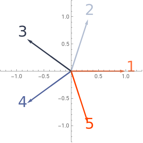
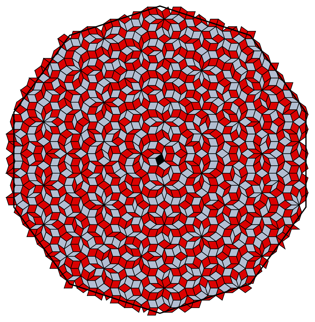
typeOfComputation=1;countGridVectors=5;withRandomVariation=False;niMax=8;
3. Computations
3. Computations
User input and preparations
User input and preparations
Line colors etc
Create some contrast between colors of neighbouring indices
Auxiliary functions
Auxiliary functions
Grid lines
Grid lines
Computation and display of the grid lines (Step 1). There are 2*niMax lines in each of the countGridVectors directions
Tiles may have been covered more than once, therefor delete duplicates:
Compute vertices of tiling (Step 3)
Compute and plot edges
Compute and plot edges
Compute corona
Compute corona
Create planar face list. This will be used for corona computation.
Delete too long element (face from outer contour):
Growth form
Growth form
v1, v2:
Intersection orthoplex - plane:
go around: