Abstract: The notion of Gravitational Waves, predicted by Albert Einstein (1916), was confirmed nearly a century later (2015). The Laser Interferometer Gravitational-Wave Observatory (LIGO) is indeed a splendid piece of engineering instrument that allows measurements of exceeding sensitivity. The primary design specification can detect strain of one part inover a 100 Hz bandwidth.
Goals: This project aims to use state-of-the-art neural networks in the wolfram language to detect to weak gravitational waves signals in presence of various white and colored noises. Further, it will be encourage to estimate the parameters of their source (the stellar-masses). Using classification and regression nets of different architecture, to detect and characterize these signals whose peak power is significantly weaker than that of the background noise.
Main results: This project allows identification of weak gravitational wave signals hidden in large data set of noise. Not only out neural net was able to verify signals inside simple white noise, it also had the capability to detect events within different types of noises and a mix of them. Lastly, by classifying the parameters into different classes, with enough training the net was able to point to the correct solar masses ranging between 5-75 solar masses with out of more than 2500 different combinations.
Future work: It will be interesting to apply these state-of-art models on real world LIGO/Virgo data to detect events in real time.
Abstract: The notion of Gravitational Waves, predicted by Albert Einstein (1916), was confirmed nearly a century later (2015). The Laser Interferometer Gravitational-Wave Observatory (LIGO) is indeed a splendid piece of engineering instrument that allows measurements of exceeding sensitivity. The primary design specification can detect strain of one part in
21
10
Goals: This project aims to use state-of-the-art neural networks in the wolfram language to detect to weak gravitational waves signals in presence of various white and colored noises. Further, it will be encourage to estimate the parameters of their source (the stellar-masses). Using classification and regression nets of different architecture, to detect and characterize these signals whose peak power is significantly weaker than that of the background noise.
Main results: This project allows identification of weak gravitational wave signals hidden in large data set of noise. Not only out neural net was able to verify signals inside simple white noise, it also had the capability to detect events within different types of noises and a mix of them. Lastly, by classifying the parameters into different classes, with enough training the net was able to point to the correct solar masses ranging between 5-75 solar masses with out of more than 2500 different combinations.
Future work: It will be interesting to apply these state-of-art models on real world LIGO/Virgo data to detect events in real time.
The Wolfram Summer School (WSS) is an intense three weeks program that allows one to conduct self independent research project using the vast Wolfram platforms, resources, language, and tools. In the WSS I received training and watched various lectures to better prepare me with the knowledge and tools to construct my research project. My project concludes of two stages, gathering and preparing the relevant data, and constructing Neural Network (NN) to analyze the data.
At first I attempted to produce a sinusoidal signal that resemble the Gravitational Waves (GW) pattern observed by two merging Binary Black-Holes (BBH), and Half way throughout the project, after reaching out to the Daniel George who worked in the Huerta group, I obtained high precision simulated GW data. This data sets were generated using arbitrarily parameters (stellar-masses) ranging from 5-75 solar masses. The first stage was to embed the original signal in white noise to imitate the disturbance associated with real LIGO/Virgo detectors. Second, we trained our NN to distinguished between input containing signal and regular noise. Later I added different noises: White, Brown, Blue, Pink, and a combination of those. Note that the training were done, separately, on both my own generated signals and the received data sets from the Huerta group. Lastly, I turned my attention parameters estimations using regression network. For this task I used the Huerta's group data and followed the same procedure including strictly white noise for multiple samples generation.
The notion of Gravitational Waves, predicted by Albert Einstein (1916), was confirmed nearly a century later (2015). The Laser Interferometer Gravitational-Wave Observatory (LIGO) is indeed a splendid piece of engineering instrument that allows measurements of exceeding sensitivity. The primary design specification can detect strain of one part inover a 100 Hz bandwidth. The Wolfram Summer School (WSS) is an intense three weeks program that allows one to conduct self independent research project using the vast Wolfram platforms, resources, language, and tools.
At first I attempted to produce a sinusoidal signal that resemble the Gravitational Waves (GW) pattern observed by two merging Binary Black-Holes (BBH), and Half way throughout the project, after reaching out to the Daniel George who worked in the Huerta group, I obtained high precision simulated GW data. This data sets were generated using arbitrarily parameters (stellar-masses) ranging from 5-75 solar masses. The first stage was to embed the original signal in white noise to imitate the disturbance associated with real LIGO/Virgo detectors. Second, we trained our NN to distinguished between input containing signal and regular noise. Later I added different noises: White, Brown, Blue, Pink, and a combination of those. Note that the training were done, separately, on both my own generated signals and the received data sets from the Huerta group. Lastly, I turned my attention parameters estimations using regression network. For this task I used the Huerta's group data and followed the same procedure including strictly white noise for multiple samples generation.
The notion of Gravitational Waves, predicted by Albert Einstein (1916), was confirmed nearly a century later (2015). The Laser Interferometer Gravitational-Wave Observatory (LIGO) is indeed a splendid piece of engineering instrument that allows measurements of exceeding sensitivity. The primary design specification can detect strain of one part in
21
10
Let us starts by looking at pure gravitational wave data. As we can see there are three main stages involved in a merge of two Binary Black Holes.
♣
The in-spiralling phase involves slow movement of the two celestial objects that can be modeled by Newtonian theory
♣
The merging phase appends very rapidly with velocities approaching the speed of light, it is modeled using numerical relativity
♣
The ring-down phase followed immediately after the merge, it characterizes by fast reducing oscillation, as echos of the merger event result from tighter and tighter spirals around the resulting black hole.
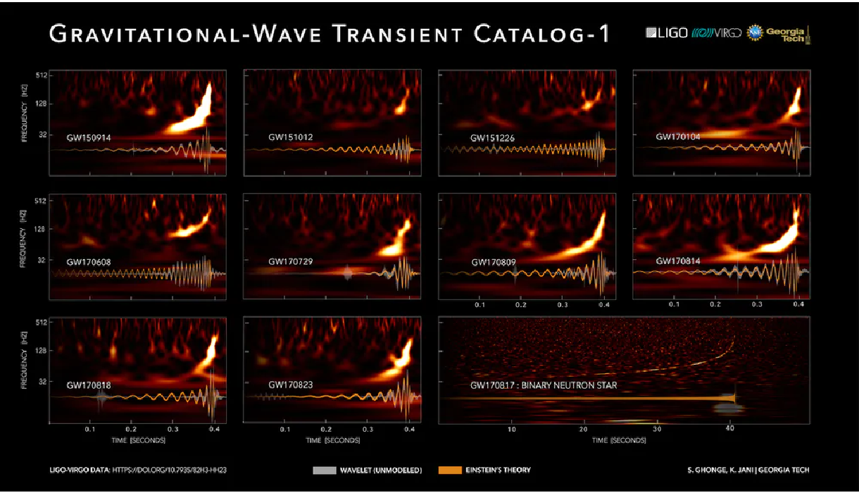
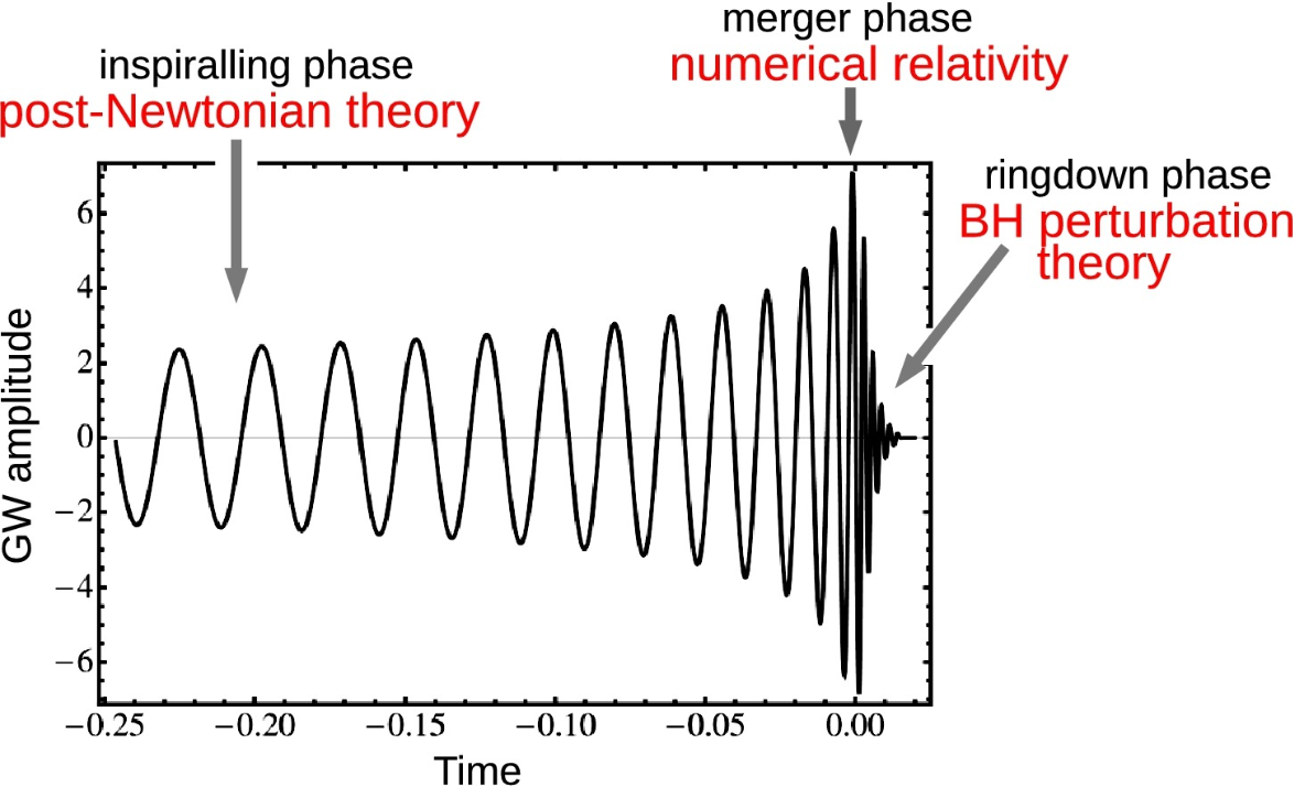
On the left, transient Catalog of Compact Binary Mergers Observed by LIGO and Virgo during the First and Second Observing Runs. On the right, the three phases of the coalescence of two compact objects (black holes).
Image credits: LIGO/VIrgo/Georgia Tech/S. Ghonge & K. Jani, and Luc Blanchet arXiv:1902.09801 respectively.
Image credits: LIGO/VIrgo/Georgia Tech/S. Ghonge & K. Jani, and Luc Blanchet arXiv:1902.09801 respectively.
Self generated data
Self generated data
At first, I attempted to produce a sinusoidal signal that resemble the Gravitational Waves (GW) pattern observed by two merging Binary Black-Holes (BBH). I used a combination of elementary functions (sinusoidal and exponential) to generate similar patterns.
Out[]=


Generating a simple list of the parameters varied according to the desired size of and accuracy, note that one can choose the size step (Δt) arbitrarily.
In[]:=
tmin=0;tmax=1;Δt=;parameters=Partition[Flatten@Table[{a->i,b->j,c->k,d->n},{i,2,2.5,0.25},{j,0.7,1.7,0.1},{k,0.4,0.7,0.05},{n,5,10,2.5}],4];values=Table[h[t]/.parameters[[i]],{i,1,Length@parameters},{t,tmin,tmax,Δt}];=WhiteNoiseProcess[];whitenoise=Table[RandomFunction[,{0,8191},2]["Path"]〚All,2〛,Length@parameters*15];
1
8191
Associating the data to its type (class) while adding white noise. The next step was to separate the data into training and testing elements where 80% is for training and the rest is for testing.
In[]:=
noised=Thread[Flatten[Table[values〚i〛+whitenoise〚j+15*(i-1)〛,{i,Length@values},{j,15}],1]"noised"];noise=Thread[Table[RandomFunction[,{0,8191},2]["Path"][[All,2]],Length@parameters*15]"noise"];data=Join[noise,noised];{trainingdata,testingdata}=TakeDrop[RandomSample[data],Floor[Length@data*0.8]];
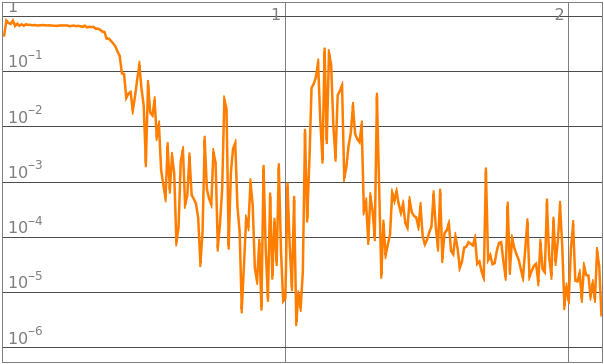
Initiate the neural net and train it on the previous data set.
Out[]=

Out[]=
NetChain


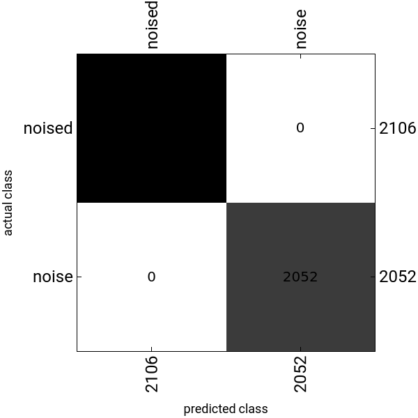
The accuracy and the confusion matrix of the testing set.
Out[]=
Designated synthetic Data
Designated synthetic Data
White noise analysis
White noise analysis
The data below is separated into three different data sets all varied both in the initial value and the margin of the Black Hole’s solar masses. The values ranged from 5-75 solar masses. Denote the pure synthetic noise as white noise and the signal plus the white noise as noised (signal). Note that the first element in the data sets is simply a list of all the signals while the second element is a list of all the weights of the Black-Holes.
In[]:=
=WhiteNoiseProcess[];noisedtraining=#+RandomFunction[,{1,8192}]["Values"]"signal"&/@trainwhiteneddata〚1〛;noisedvalidate=#+RandomFunction[,{1,8192}]["Values"]"signal"&/@validatewhiteneddata〚1〛;noisedtest=#+RandomFunction[,{1,8192}]["Values"]"signal"&/@testwhiteneddata〚1〛;
In[]:=
noise=Table[RandomFunction[,{1,8192}]["Values"]"noise",14769];data=Join[noisedtraining,noisedvalidate,noisedtest,noise];{train,test}=TakeDrop[RandomSample[data],Floor[Length@data*0.75]];{train,validate}=TakeDrop[RandomSample[train],Floor[Length@train*0.9]];
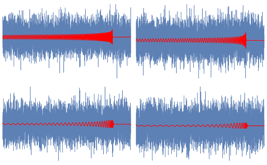
Initiate the neural net and train after declaring the previous data set.
Out[]=
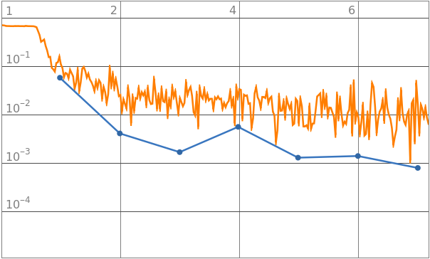
The accuracy and the confusion matrix of the testing set.
Brown noise analysis
Brown noise analysis
The data below is separated into three different data sets all varied both in the initial value and the margin of the Black Hole’s solar masses. The values ranged from 5-75 solar masses. Denote the pure synthetic noise as white noise and the signal plus the white noise as noised (signal). Note that the first element in the data sets is simply a list of all the signals while the second element is a list of all the weights of the Black-Holes.
Initiate the neural net and train after declaring the previous data set.
The accuracy and the confusion matrix of the testing set.
Multiple noise analysis
Multiple noise analysis
The data below is separated into three different data sets all varied both in the initial value and the margin of the Black Hole’s solar masses. The values ranged from 5-75 solar masses. Denote the pure synthetic noise as white noise and the signal plus the white noise as noised (signal). Note that the first element in the data sets is simply a list of all the signals while the second element is a list of all the weights of the Black-Holes.
This part uses white, brown, blue, and pink noises
Adding the noise to each data set. We mixed all the noises and rearranged them in random order, then they were added to the signals and assigned the class “signal”.
Initiate the neural net and train after declaring the previous data set.
The accuracy and the confusion matrix of the testing set.
Parameter Estimation
Parameter Estimation
The data below is separated into three different data sets all varied both in the initial value and the margin of the Black Hole’s solar masses. The values ranged from 5-75 solar masses. Denote the pure synthetic noise as white noise and the signal plus the white noise as noised (signal). Note that the first element in the data sets is simply a list of all the signals while the second element is a list of all the weights of the Black-Holes.
Generating 50 different white noised data fore each signal and associating them to the relevant parameters. Note that only a portion of the data is taken because of computational limitations and time constrains.
In this stage because of the variety of classes, over 2500, the signal to noise ratio was to cumbersome to work with. The white noise has to be truncated to 30% compared to previous examples.
The next step is to get the solar masses from the indexed number, for that we build a dictionary. this makes the work easier, one simply has to use v-lookup on the output from given by the neural net and the index will indicate the desire parameter values.
Initiate the neural net and train after declaring the previous data set.
The accuracy of the trained neural net on the testing set. These results are quite remarkable because the network has over 2500 classes to choose from.
Acknowledgment
Acknowledgment
Mentor: Tuseeta Banerjee
This project could have not been done without the help and dedication of my mentor Tuseeta Banerjee. The knowledge and skills she possess in the field helped me avoid many mistakes along the way. Moreover, her warm and welcoming personality had made this project fun and engaging. Another essential individual to acknowledge is Daniel George who was extremely kind to share his knowledge and his group data sets. Without both of them I could have not reach my goals and finish the project.
References
References
◼
D. George and E. A. Huerta. Deep neural networks to enable real-time multimessenger astrophysics. Phys. Rev. D, 97:044039, Feb 2018.
◼
D. George and E. A. Huerta. Deep Learning for real-time gravitational wave detection and parameter estimation: Results with Advanced LIGO data. Physics Letters B, 778:64 – 70, 2018.
◼
L. Blanchet. Analyzing Gravitational Waves with General Relativity, Comptes Rendus Physique 20 (2019) 507-520