Liquid chromatography is a common technique in analytical chemistry used to identify and quantify chemical species in a mixture. The mixture is injected at the inlet of a chromatographic column and a liquid mobile phase (the solvent) allows their elution. The liquid chromatography technique is based on the difference in adsorption of the chemicals on a solid stationary phase or adsorbent. Hence, different chemical species will elute at different retention times.
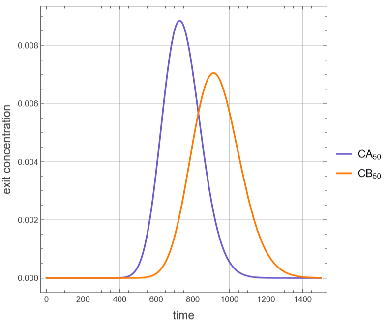
In this notebook, two components (A and B) are separated by liquid chromatography using the stagewise model. This model considers the chromatographic column to be a series of 50 well-mixed stirred tanks or 50 perfect equilibrium stages. Linear adsorption isotherms with equilibrium constants are assumed for this stagewise model. The two peaks at the exit of the column are plotted. These peaks are symmetric because of the linear equilibrium hypothesis. The order of elution of the two components depends on the relative values of their equilibrium constants, which can be varied. Due to dispersion, peaks get broader and smaller for larger elution times.
In this notebook, two components (A and B) are separated by liquid chromatography using the stagewise model. This model considers the chromatographic column to be a series of 50 well-mixed stirred tanks or 50 perfect equilibrium stages. Linear adsorption isotherms with equilibrium constants are assumed for this stagewise model. The two peaks at the exit of the column are plotted. These peaks are symmetric because of the linear equilibrium hypothesis. The order of elution of the two components depends on the relative values of their equilibrium constants, which can be varied. Due to dispersion, peaks get broader and smaller for larger elution times.
Equilibrium constants
KA=0.9;KB=1.3;
Total volume
V
tot
50 well-mixed stirred tanks or 50 perfect equilibrium stages
NS=50;
Stage volume
V
stage
V
tot
Base case - sloppy separation
Base case - sloppy separation
Volumetric flow rate
L=0.4;
Void fraction
ϵ=0.4;
Column diameter
Dc=4;
Column length
Lbed=25;
In[]:=
eq[i_]:=D[[t],{t,1}]L([t]-[t])ϵ+(1-ϵ)KA;eq2[i_]:=D[[t],{t,1}]L([t]-[t])ϵ+(1-ϵ)KB;eqn=Table[eq[i],{i,1,50}];
CA
i
CA
i-1
CA
i
V
stage
V
stage
CB
i
CB
i-1
CB
i
V
stage
V
stage
In[]:=
initialCond=Table[[0]0,{i,1,50}];sys=Flatten[Join[eqn,initialCond]];Unknown=Table[,{i,1,50}];eqn2=Table[eq2[i],{i,1,50}];initialCond2=Table[[0]0,{i,1,50}];sys2=Flatten[Join[eqn2,initialCond2]];Unkn2=Table[,{i,1,50}];
CA
i
CA
i
CB
i
CB
i
In[]:=
CA
0
CA
init
CA
init
CB
0
CB
init
CB
init
In[]:=
sol1=NDSolve[sys,Unknown,{t,0,5000}];sol2=NDSolve[sys2,Unkn2,{t,0,3000}];
plt2=Plot{Evaluate[[t]]/.sol1,Evaluate[[t]]/.sol2},{t,0,1500},
CA
50
CB
50
Out[]=
Resolution (Rs) separation criterion
Resolution (Rs) separation criterion
Match the upper t-limit used in NDSolve/Plot for this case
tmax=2000;
In[]:=
cA[t_]:=Evaluate[[t]]/.sol1[[1]]cB[t_]:=Evaluate[[t]]/.sol2[[1]]
CA
50
CB
50
Zeroth moment: area under each peak
areaA=NIntegrate[cA[t],{t,0,tmax}];areaB=NIntegrate[cB[t],{t,0,tmax}];
First moment: retention time (mean elution time)
tRA=NIntegrate[t*cA[t],{t,0,tmax}]/areaA;tRB=NIntegrate[t*cB[t],{t,0,tmax}]/areaB;
Second central moment: variance->sigma
varA=NIntegrate[(t-tRA)^2*cA[t],{t,0,tmax}]/areaA;varB=NIntegrate[(t-tRB)^2*cB[t],{t,0,tmax}]/areaB;sigmaA=Sqrt[varA];sigmaB=Sqrt[varB];
Baseline peak width, Gaussian approx: w=4*sigma
wA=4*sigmaA;wB=4*sigmaB;
Resolution
Rs=2*(tRB-tRA)/(wA+wB);Print["Retention time A = ",NumberForm[tRA,5]];Print["Retention time B = ",NumberForm[tRB,5]];Print["Peak width A (4σ) = ",NumberForm[wA,5]];Print["Peak width B (4σ) = ",NumberForm[wB,5]];Print["Resolution Rs = ",NumberForm[Rs,4]];
Retention time A = 743.27
Retention time B = 931.77
Peak width A (4σ) = 417.79
Peak width B (4σ) = 524.38
Resolution Rs = 0.4001
Case study 2 - lower the volumetric flow rate to improve the separation
Case study 2 - lower the volumetric flow rate to improve the separation
Volumetric flow rate
L=0.1;
Void fraction
ϵ=0.4;
Column diameter
Dc=4;
Column length
Lbed=25;
In[]:=
initialCond=Table[[0]0,{i,1,50}];sys=Flatten[Join[eqn,initialCond]];Unknown=Table[,{i,1,50}];sol1=NDSolve[sys,Unknown,{t,0,6000}];eqn2=Table[eq2[i],{i,1,50}];initialCond2=Table[[0]0,{i,1,50}];sys2=Flatten[Join[eqn2,initialCond2]];Unkn2=Table[,{i,1,50}];sol2=NDSolve[sys2,Unkn2,{t,0,6000}];
CA
i
CA
i
CB
i
CB
i
plt2=Plot{Evaluate[[t]]/.sol1,Evaluate[[t]]/.sol2},{t,0,6000},
CA
50
CB
50
Out[]=
Resolution (Rs) separation criterion
Resolution (Rs) separation criterion
Match the upper t-limit used in NDSolve/Plot for this case
Zeroth moment: area under each peak
First moment: retention time (mean elution time)
Second central moment: variance->sigma
Baseline peak width, Gaussian approx: w=4*sigma
Resolution
Case study 3 - increase the column length to improve the separation
Case study 3 - increase the column length to improve the separation
Volumetric flow rate
Void fraction
Column diameter
Column length
Resolution (Rs) separation criterion
Resolution (Rs) separation criterion
Match the upper t-limit used in NDSolve/Plot for this case
Zeroth moment: area under each peak
First moment: retention time (mean elution time)
Second central moment: variance->sigma
Baseline peak width, Gaussian approx: w=4*sigma
Resolution
Case study 4 - narrower injection won’t help
Case study 4 - narrower injection won’t help
Volumetric flow rate
Void fraction
Column diameter
Column length
Resolution (Rs) separation criterion
Resolution (Rs) separation criterion
Match the upper t-limit used in NDSolve/Plot for this case
Zeroth moment: area under each peak
First moment: retention time (mean elution time)
Second central moment: variance->sigma
Baseline peak width, Gaussian approx: w=4*sigma
Resolution
Case study 5 - increase number of stages
Case study 5 - increase number of stages
Volumetric flow rate
Void fraction
Column diameter
Column length
Equilibrium constants
Total volume
200 well-mixed stirred tanks or 200 perfect equilibrium stages
Stage volume
Resolution (Rs) separation criterion
Resolution (Rs) separation criterion
Match the upper t-limit used in NDSolve/Plot for this case
Zeroth moment: area under each peak
First moment:retention time (mean elution time)
Second central moment: variance->sigma
Baseline peak width, Gaussian approx: w=4*sigma
Resolution
Case study 6 - change equilibrium constants
Case study 6 - change equilibrium constants
Equilibrium constants
Total volume
50 well-mixed stirred tanks or 50 perfect equilibrium stages
Stage volume
Volumetric flow rate
Void fraction
Column diameter
Column length
Resolution (Rs) separation criterion
Resolution (Rs) separation criterion
Match the upper t-limit used in NDSolve/Plot for this case
Zeroth moment: area under each peak
First moment:retention time (mean elution time)
Second central moment: variance->sigma
Baseline peak width,Gaussian approx: w=4*sigma
Resolution
Discussion
Discussion
The five case studies above each change a single operating or design parameter of the stagewise (plate) chromatography model relative to the base case (L = 0.4, Lbed = 25, NS = 50, KA = 0.9, KB = 1.3, injection width = 10), which gives a poor resolution of Rs = 0.40. Comparing retention times, peak widths (4-sigma) and resolution across the cases shows how each parameter acts through one of the three classic levers of a chromatographic separation: retention/capacity, selectivity, and column efficiency.
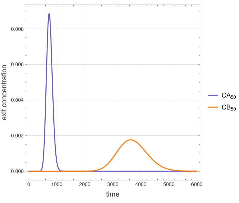
Case study 2 - lower flow rate: Reducing the volumetric flow rate L from 0.4 to 0.1 (one quarter of the base case) leaves the retention time of the weakly retained species A essentially unchanged (about 743 time units), but delays the more strongly retained species B considerably, from about 932 to about 3712 time units. Peak B also broadens substantially, from about 524 to about 2095, yet the extra separation between the peaks more than compensates for this broadening: the resolution rises from Rs = 0.40 to Rs = 2.36, essentially a baseline separation of the two components. The cost is a nearly four-fold increase in total run time, which is the classic trade-off between resolution and analysis time/throughput when flow rate is the tuning parameter.
Case study 3 - increase column length: Lengthening the packed bed from 25 to 45 cm at the original flow rate again leaves the retention time of A close to 743, while the retention time of B increases to about 1673 and peak B broadens to about 944. The resolution improves to Rs = 1.37, better than the base case but a smaller gain than the one obtained by lowering the flow rate in case study 2. A longer column is therefore also an effective way to improve the separation, but for a comparable increase in elution/analysis time it delivers less resolution than reducing the flow rate, and it additionally requires more packing material and a larger column.
Case study 4 - narrower injection: Shrinking the injection pulse width by a factor of 100, from 10 to 0.1 time units, barely changes anything: the retention times, both peak widths, and the resolution (Rs = 0.399, essentially the same as the base-case value of 0.40) are almost identical to the base case. This confirms the title of the case study - narrowing the injection has almost no effect here because, in this 50-stage plate model, band broadening is governed by the finite number of equilibrium stages built into the stagewise model, not by the width of the injected pulse. Once the column's own dispersion dominates the peak shape, sharpening the injection cannot meaningfully improve the separation.
Case study 5 - increase number of stages: Quadrupling the number of equilibrium stages from 50 to 200 leaves both retention times essentially unchanged, as expected since retention time depends on the equilibrium constants and the phase ratio rather than on the number of stages, but it nearly halves both peak widths (peak A: about 418 down to about 209; peak B: about 524 down to about 262). As a result, the resolution doubles, from Rs = 0.40 to Rs = 0.80. This is the classic plate-theory result: peak width scales approximately as 1 over the square root of the number of stages, and resolution scales approximately as the square root of the number of stages, so adding stages sharpens the peaks without shifting where they elute.
Case study 6 - change equilibrium constants: Increasing the equilibrium constant of B from 1.3 to 3.3, while keeping the equilibrium constant of A fixed at 0.9, raises the selectivity between the two solutes: the ratio of equilibrium constants grows from about 1.4 to about 3.7. The retention time of A is unaffected (about 743), while B now elutes much later, at about 1874 instead of about 932, and peak B widens to about 1057. The resolution jumps to Rs = 1.53. Because the equilibrium constants reflect the underlying chemistry of the adsorbent and mobile phase, this case shows that changing the stationary or mobile phase to alter the relative affinities of the solutes is one of the most powerful ways to improve a separation, more effective in this comparison than doubling the column length in case study 3.
Summary: Ranking the five modifications by the resolution they achieve gives: lowering the flow rate, Rs = 2.36 (case 2); increasing the equilibrium constant of B, Rs = 1.53 (case 6); increasing the column length, Rs = 1.37 (case 3); increasing the number of stages, Rs = 0.80 (case 5); and narrowing the injection, Rs = 0.40, no improvement over the base case (case 4). This ordering illustrates the classical resolution equation of chromatography, in which resolution depends on the retention factor, the selectivity between the two solutes, and the column efficiency (number of theoretical plates). Acting on selectivity or on retention, by changing the flow rate, the column length, or the equilibrium constants, tends to give the largest gains in resolution, while increasing efficiency alone, by adding stages, gives a smaller, square-root-law improvement, and reducing the injection width gives essentially no benefit once the column's intrinsic dispersion already dominates the peak shape. In practice, the choice between these levers also involves a trade-off with analysis time, amount of packing material, and the chemistry of the stationary/mobile phase pair that is available.
Reference
Reference
[1] J. Ingham, I. J. Dunn, E. Heinzle, and J. E. Prenosil, “CHROMPLATE - Stagewise Model for Chromatography Columns,” Chemical Engineering Dynamics, 2nd ed., Weinheim, Germany: Wiley-VCH, 500 pp. 541–545.
CITE THIS NOTEBOOK
CITE THIS NOTEBOOK
Liquid chromatography with linear adsorption equilibrium and plate model
by Housam Binous
Wolfram Community, STAFF PICKS, August 10, 2026
https://community.wolfram.com/groups/-/m/t/3778307
by Housam Binous
Wolfram Community, STAFF PICKS, August 10, 2026
https://community.wolfram.com/groups/-/m/t/3778307