Abstract: In this project we want to investigate the quantum spin chain models with multiway system, and explore the connection between the multiway system and the tensor network.
Quantum Transverse Field Ising Model Hamiltonian
Quantum Transverse Field Ising Model Hamiltonian
Implement the quantum transverse Ising model Hamiltonian and convert the quantum system’s evolution to a multiway system.
Introduction
Introduction
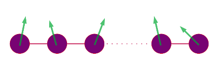
The 1 D quantum transverse field Ising model’s Hamiltonian is
Out[]=
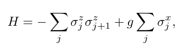
where are the Pauli operators, g is the transverse magnetic field strength. Based on the Schrödinger equation we have
x,y,z
σ
Out[]=
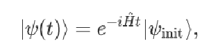
and this evolution dynamics for a quantum state can be mapped to a multiway system using QuantumToMultiwaySystem (see Wolfram function repository for more details).
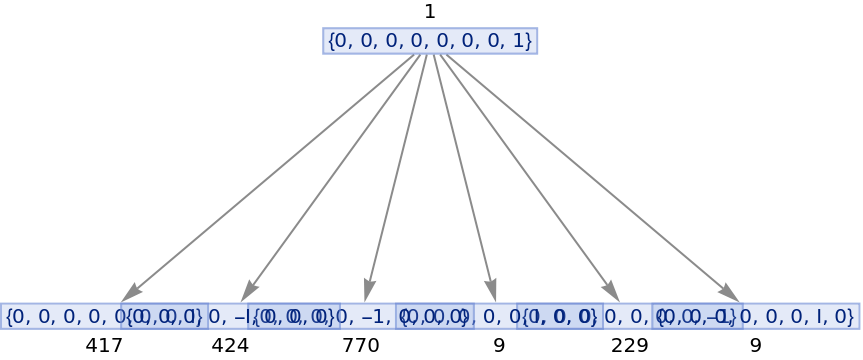
The initial state is expanded in the given basis, while the evolution operator is transformed to the rule for multiway system.
The initial state is expanded in the given basis, while the evolution operator is transformed to the rule for multiway system.
Quantum Evolution
Quantum Evolution
An initial quantum state for a spin chain is evolved under a Hamiltonian, and this is the quench dynamics for the quantum system.
Quantum Ising model Hamiltonian matrix. n is the spin number, g is the parameter.
In[]:=
Ho1[oper1_,iden_,stringN_,i_]:=Module[{opList=Table[iden,{stringN}]},opList〚i〛=oper1;Fold[KroneckerProduct[#1,#2]&,opList〚1〛,opList〚2;;〛]]Ho2[oper1_,oper2_,iden_,stringN_,i_]:=Module[{opList=Table[iden,{stringN}]},opList[[i]]=oper1;opList[[i+1]]=oper2;Fold[KroneckerProduct[#1,#2]&,opList[[1]],opList[[2;;]]]]Ham[n_,g_]:=Module[{σx={{0,1},{1,0}},σy={{0,-I},{I,0}},σz={{1,0},{0,-1}},iden={{1,0},{0,1}},Hx,Hz},Hx=Ho1[g*σx,iden,n,0];Hx=Hx+Total[Ho1[g*σx,iden,n,#]&/@Range[2,n]];Hz=Ho2[-σz,σz,iden,n,0];Hz=Hz+Total[Ho2[-σz,σz,iden,n,#]&/@Range[2,n-1]];Hz+Hx]
Here we only consider 3 spins. The parameter $g=2$, evolution time $t=1$.
n=3;g=1.5;evoIsing=N@MatrixExp[-I*Ham[n,g]]
Out[]=
{{0.475206+0.0351769,0.00892117-0.00408284,0.00892117-0.00408284,-0.065096+0.876648,0.+0.,0.+0.,0.+0.,0.+0.},{0.00892117-0.00408284,-0.283994+0.382631,0.705999+0.523751,0.00892117-0.00408284,0.+0.,0.+0.,0.+0.,0.+0.},{0.00892117-0.00408284,0.705999+0.523751,-0.283994+0.382631,0.00892117-0.00408284,0.+0.,0.+0.,0.+0.,0.+0.},{-0.065096+0.876648,0.00892117-0.00408284,0.00892117-0.00408284,0.475206+0.0351769,0.+0.,0.+0.,0.+0.,0.+0.},{0.+0.,0.+0.,0.+0.,0.+0.,-0.229742+0.417465,4.77049×+0.00981106,9.54098×+0.00981106,-0.770044-0.424006},{0.+0.,0.+0.,0.+0.,0.+0.,-4.25007×+0.00981106,-0.229742-0.417465,-0.770044+0.424006,3.20924×+0.00981106},{0.+0.,0.+0.,0.+0.,0.+0.,-7.11237×+0.00981106,-0.770044+0.424006,-0.229742-0.417465,1.9082×+0.00981106},{0.+0.,0.+0.,0.+0.,0.+0.,-0.770044-0.424006,-8.67362×+0.00981106,-5.11743×+0.00981106,-0.229742+0.417465}}
-17
10
-17
10
-17
10
-17
10
-17
10
-17
10
-17
10
-17
10
In[]:=
evoIsing=IntegerPart[1000*evoIsing](*t=1*)(*Enlargethevolutionoperatortosatisfythefunctionrequrement.*)
Out[]=
{{475+35,8-4,8-4,-65+876,0,0,0,0},{8-4,-283+382,705+523,8-4,0,0,0,0},{8-4,705+523,-283+382,8-4,0,0,0,0},{-65+876,8-4,8-4,475+35,0,0,0,0},{0,0,0,0,-229+417,9,9,-770-424},{0,0,0,0,9,-229-417,-770+424,9},{0,0,0,0,9,-770+424,-229-417,9},{0,0,0,0,-770-424,9,9,-229+417}}
Product State 1
Product State 1
Initial quantum state:
In[]:=
sList=Table[{0,1},{n}]initIsing1=Fold[Flatten[KroneckerProduct[#1,#2]]&,sList[[1]],sList[[2;;]]]
Out[]=
{{0,1},{0,1},{0,1}}
Out[]=
{0,0,0,0,0,0,0,1}
In[]:=
ResourceFunction["QuantumToMultiwaySystem"][evoIsing,initIsing1,1,"EvolutionGraph","IncludeStatePathWeights"True,VertexLabels"VertexWeight"]
Out[]=
In[]:=
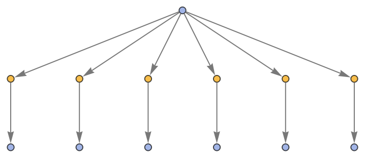
ResourceFunction["QuantumToMultiwaySystem"][evoIsing,initIsing1,1,"EvolutionCausalGraphStructure"]
Out[]=
In[]:=
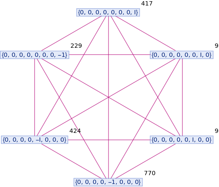
ResourceFunction["QuantumToMultiwaySystem"][evoIsing,initIsing1,1,"BranchialGraph","IncludeStatePathWeights"True,VertexLabels->"VertexWeight"]
Out[]=
Product State 2
Product State 2
sList={{2,1},{1,1},{1,4}}initIsing2=Fold[Flatten[KroneckerProduct[#1,#2]]&,sList[[1]],sList[[2;;]]](*Notethatwedon'tconsiderthewavefunctionnormalizationhere,becarefulwhenyoustudyphysicsrelatedwiththisissue*)
Out[]=
{{2,1},{1,1},{1,4}}
Out[]=
{2,8,2,8,1,4,1,4}
In[]:=
ResourceFunction["QuantumToMultiwaySystem"][evoIsing,initIsing2,1,"EvolutionGraph","IncludeStatePathWeights"True,VertexLabels"VertexWeight"]
Out[]=

In[]:=
ResourceFunction["QuantumToMultiwaySystem"][evoIsing,initIsing2,1,"BranchialGraphStructure","IncludeStatePathWeights"True,VertexLabels->"VertexWeight"]
Entangled State
Entangled State
Multiway Many-Body Physics
Multiway Many-Body Physics
The quantum evolution for an initial state can be expressed by a multiway system, however, we cannot know the local Hilbert space’s information just through the QuantumToMultiwaySystem translation. Here we want to explore the many-body physics.
Consider a two local spin system and assume two local Hamiltonian is commutative. The evolution operator is the tensor product of two local evolution operator.
Here we use two general matrix (without the unitarity requirement for the evolution operator) to study the general updating process.
Concluding remarks
Concluding remarks
The quantum evolution dynamics can be translated to a multiway system. For a quantum many-body system, the intriguing entanglement property may be decoded from the multiway system. Here we are just starting to explore the quantum many-body physics from the perspective of multiway system.
From the geometric property of the branchial graph, some interesting information about the many-body system may be uncovered. However, I haven’t find a method to achieve this goal.
Later, we will continue to deepen the study about the multiway system’s many-body physics.
From the geometric property of the branchial graph, some interesting information about the many-body system may be uncovered. However, I haven’t find a method to achieve this goal.
Later, we will continue to deepen the study about the multiway system’s many-body physics.
Keywords
Keywords
◼
Multiway system
◼
Quantum many-body physics
◼
Geometric information
Acknowledgment
Acknowledgment
The author would like to thank Stephen Wolfram and Jonathan Gorard for introducing this attractive project and help during the summer school. And thank my mentor Jack Heimrath very much. Jack helps me a lot during the whole summer school. Thanks all TAs and speakers for help and amazing talks. I want to thank Erin Cherry, Danielle Rommel Mayer and Hatem Elshatlawy for ther kindful help. At last thanks all other staff members and students.
References
References
◼
[1] S. Wolfram (2002), A New Kind of Science. Champaign, Illinois: Wolfram Media, Inc. https://www.wolframscience.com/nks
◼
[2] J. Gorard (2020), “Some Quantum Mechanical Properties of the Wolfram Model”, Complex Systems 29 (2): 537-598. https://www.complex-systems.com/abstracts/v29_i02_a02/