We compute the stripping and rectifying composition profiles of an ideal ternary mixture at atmospheric pressure. The mixture consists of three components:
Pentane = component 1
Hexane = component 2
Heptane = component 3
The constant relative volatilities are taken equal to 6.35 and 2.47.
Pentane = component 1
Hexane = component 2
Heptane = component 3
The constant relative volatilities are taken equal to 6.35 and 2.47.
For ternary systems with constant relative volatilities, we have the following relation between liquid and vapor mole fractions :=, where (i.e., component 3 is the reference component).
y
i
α
ik
x
i
3
∑
j=1
α
jk
x
j
k=3
The reflux and reboil ratios are set equal to 2.5 and 1.35, respectively. Feed is saturated liquid with the following composition : 30% Pentane, 30% Hexane, 40% Heptane. Additional specifications are as follows:
Distillate composition: 95% Pentane, 4.9% Hexane, 0.1% Heptane and Bottom composition: 5% Pentane.
Distillate composition: 95% Pentane, 4.9% Hexane, 0.1% Heptane and Bottom composition: 5% Pentane.
We successfully reproduce Fig. 4.2 of Ref. 1.
Overall Material Balance gives Bottom composition:
5% Pentane, 39.7% Hexane, 55.3% Heptane
Without loss of generality, we take F = feed flow rate = 1 kmol/hr as a basis.
5% Pentane, 39.7% Hexane, 55.3% Heptane
Without loss of generality, we take F = feed flow rate = 1 kmol/hr as a basis.
In[]:=
F=1;
In[]:=
FindRoot[{FDist+B,F0.3Dist0.95+B0.05,F0.3Dist0.049+BHBottom},{B,1},{Dist,0.8},{HBottom,0.7}]
Out[]=
{B0.722222,Dist0.277778,HBottom0.396538}
Calculation of the liquid composition profile in the Rectifying Section with 10 Stages. Reflux ratio is equal to 2.5.
In[]:=
r=2.5;(*refluxratio*)
In[]:=
d[1]=0.95;d[2]=0.049;d[3]=0.001;(*distillatecomposition*)Ne=10;(*numberofstages*)
In[]:=
xr[1,Ne]=0.95;xr[2,Ne]=0.049;xr[3,Ne]=0.001;
In[]:=
Rect[i_,n_]:=yr[i,n-1]r/(r+1)xr[i,n]+d[i]/(r+1)(*rectifyingsectionoperatingline*)
In[]:=
a[1]=6.35;a[2]=2.47;a[3]=1;(*relativevolatilities*)
In[]:=
sol=NSolve[{xr[1,Ne]a[1]xr[1,Ne-1]/Sum[a[j]xr[j,Ne-1],{j,1,3}],xr[2,Ne]a[2]xr[2,Ne-1]/Sum[a[j]xr[j,Ne-1],{j,1,3}],1Sum[xr[j,Ne-1],{j,1,3}]},{xr[1,Ne-1],xr[2,Ne-1],xr[3,Ne-1]}]
Out[]=
{{xr[1,9]0.877743,xr[2,9]0.11639,xr[3,9]0.00586702}}
In[]:=
xr[1,Ne-1]=sol[[1,1,2]]
Out[]=
0.877743
In[]:=
xr[2,Ne-1]=sol[[1,2,2]]
Out[]=
0.11639
In[]:=
xr[3,Ne-1]=sol[[1,3,2]]
Out[]=
0.00586702
In[]:=
Eq1[i_,n_]:=xr[i,n]yr[i,n]/a[i]1/Sum[yr[j,n]/a[j],{j,1,3}](*equilibriumrelations*)
In[]:=
Sys1=Table[Rect[i,n],{i,1,3},{n,1,Ne-1}];
In[]:=
Sys2=Table[Eq1[i,n],{i,1,3},{n,0,Ne-2}];
In[]:=
System1=Flatten[Join[Sys1,Sys2]];
In[]:=
unk1=Table[{xr[i,n],0.2},{i,1,3},{n,0,Ne-2}];
In[]:=
unk2=Table[{yr[i,n],0.5},{i,1,3},{n,0,Ne-2}];
In[]:=
Unknown1=Flatten[Join[unk1,unk2],1];
In[]:=
sol1=FindRoot[System1,Unknown1]
Out[]=
{xr[1,0]0.0727197,xr[1,1]0.0753328,xr[1,2]0.0821565,xr[1,3]0.100303,xr[1,4]0.146924,xr[1,5]0.249391,xr[1,6]0.415408,xr[1,7]0.603285,xr[1,8]0.763588,xr[2,0]0.0209134,xr[2,1]0.031336,xr[2,2]0.0551776,xr[2,3]0.105876,xr[2,4]0.196749,xr[2,5]0.308242,xr[2,6]0.362805,xr[2,7]0.314442,xr[2,8]0.212252,xr[3,0]0.906367,xr[3,1]0.893331,xr[3,2]0.862666,xr[3,3]0.793822,xr[3,4]0.656327,xr[3,5]0.442367,xr[3,6]0.221787,xr[3,7]0.0822734,xr[3,8]0.0241603,yr[1,0]0.325238,yr[1,1]0.330112,yr[1,2]0.343073,yr[1,3]0.376374,yr[1,4]0.449565,yr[1,5]0.568149,yr[1,6]0.702346,yr[1,7]0.816848,yr[1,8]0.898388,yr[2,0]0.0363828,yr[2,1]0.0534126,yr[2,2]0.0896254,yr[2,3]0.154535,yr[2,4]0.234173,yr[2,5]0.273146,yr[2,6]0.238601,yr[2,7]0.165609,yr[2,8]0.0971359,yr[3,0]0.638379,yr[3,1]0.616476,yr[3,2]0.567301,yr[3,3]0.469091,yr[3,4]0.316262,yr[3,5]0.158705,yr[3,6]0.0590525,yr[3,7]0.0175431,yr[3,8]0.00447644}
In[]:=
Do[xr[1,i]=(xr[1,i]/.sol1),{i,0,9}]
In[]:=
Do[xr[2,i]=(xr[2,i]/.sol1),{i,0,9}]
In[]:=
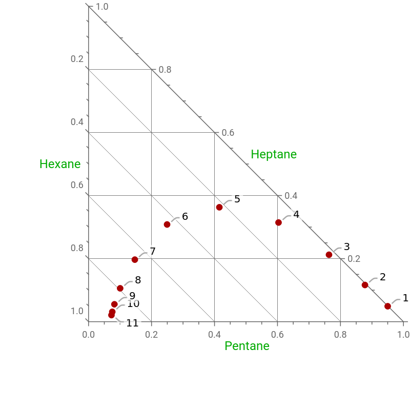
tbl1=Table[{xr[1,i],xr[2,i],1-xr[1,i]-xr[2,i]},{i,0,Ne}]
Out[]=
{{0.0727197,0.0209134,0.906367},{0.0753328,0.031336,0.893331},{0.0821565,0.0551776,0.862666},{0.100303,0.105876,0.793822},{0.146924,0.196749,0.656327},{0.249391,0.308242,0.442367},{0.415408,0.362805,0.221787},{0.603285,0.314442,0.0822734},{0.763588,0.212252,0.0241603},{0.877743,0.11639,0.00586702},{0.95,0.049,0.001}}
In[]:=
Length[tbl1]
Out[]=
11
Rectifying profile. The points’ labels indicate the stage number (we count starting from the top).
In[]:=
plt1=TernaryListPlot[Reverse@tbl1->Range[11],PlotRange{{0,1},{0,1}},AspectRatio1,GridLines->Automatic,TernaryPlotCorners->{{0,0},{1,0},{0,1}},PlotStyle->{{PointSize[0.02],Darker@Red}},GridLinesStyle->Darker[Gray],FrameLabel{Style[" Pentane",12,Darker@Green],Style[" Heptane",12,Darker@Green],Style[" Hexane",12,Darker@Green]},ImageSize->400{1,1},ImagePadding->{{80,0},{80,0}}]
Out[]=
In[]:=
plt1b=TernaryListPlot[Reverse@Drop[tbl1,5]->Range[6],PlotRange{{0,1},{0,1}},AspectRatio1,GridLines->Automatic,TernaryPlotCorners->{{0,0},{1,0},{0,1}},Joined->True,PlotStyle->{Darker@Red,Thick},PlotMarkers->Style["●",Darker@Red,12],GridLinesStyle->Darker[Gray],FrameLabel{Style[" Pentane",12,Darker@Green],Style[" Heptane",12,Darker@Green],Style[" Hexane",12,Darker@Green]},ImageSize->400{1,1},ImagePadding->{{80,0},{80,0}}];
Calculation of the liquid composition profile in the Stripping Section with 10 Stages. Reboil ratio is eaqual to 1.35.
In[]:=
S[i_,n_]:=ys[i,n](s+1)/sxs[i,n+1]-b[i]/s(*strippingsectionoperatingline*)
In[]:=
b[1]=0.05;b[2]=0.397;b[3]=0.553;(*bottomcomposition*)
In[]:=
s=1.35;(*reboilratio*)
In[]:=
Do[{xs[i,0]=b[i]},{i,1,3}];
In[]:=
Sys3=Table[S[i,n],{i,1,3},{n,0,Ne-1}];
In[]:=
Eq2[i_,n_]:=ys[i,n]xs[i,n]a[i]1/Sum[xs[j,n]a[j],{j,1,3}](*equilibriumrelations*)
In[]:=
Sys4=Table[Eq2[i,n],{i,1,3},{n,0,Ne-1}];
In[]:=
System2=Flatten[Join[Sys3,Sys4]];
In[]:=
unk3=Table[{xs[i,n],0.2},{i,1,3},{n,1,Ne}];
In[]:=
unk4=Table[{ys[i,n],0.5},{i,1,3},{n,0,Ne-1}];
In[]:=
Unknown2=Flatten[Join[unk3,unk4],1]
Out[]=
{{xs[1,1],0.2},{xs[1,2],0.2},{xs[1,3],0.2},{xs[1,4],0.2},{xs[1,5],0.2},{xs[1,6],0.2},{xs[1,7],0.2},{xs[1,8],0.2},{xs[1,9],0.2},{xs[1,10],0.2},{xs[2,1],0.2},{xs[2,2],0.2},{xs[2,3],0.2},{xs[2,4],0.2},{xs[2,5],0.2},{xs[2,6],0.2},{xs[2,7],0.2},{xs[2,8],0.2},{xs[2,9],0.2},{xs[2,10],0.2},{xs[3,1],0.2},{xs[3,2],0.2},{xs[3,3],0.2},{xs[3,4],0.2},{xs[3,5],0.2},{xs[3,6],0.2},{xs[3,7],0.2},{xs[3,8],0.2},{xs[3,9],0.2},{xs[3,10],0.2},{ys[1,0],0.5},{ys[1,1],0.5},{ys[1,2],0.5},{ys[1,3],0.5},{ys[1,4],0.5},{ys[1,5],0.5},{ys[1,6],0.5},{ys[1,7],0.5},{ys[1,8],0.5},{ys[1,9],0.5},{ys[2,0],0.5},{ys[2,1],0.5},{ys[2,2],0.5},{ys[2,3],0.5},{ys[2,4],0.5},{ys[2,5],0.5},{ys[2,6],0.5},{ys[2,7],0.5},{ys[2,8],0.5},{ys[2,9],0.5},{ys[3,0],0.5},{ys[3,1],0.5},{ys[3,2],0.5},{ys[3,3],0.5},{ys[3,4],0.5},{ys[3,5],0.5},{ys[3,6],0.5},{ys[3,7],0.5},{ys[3,8],0.5},{ys[3,9],0.5}}
In[]:=
Length[Unknown2]
Out[]=
60
In[]:=
Length[System2]
Out[]=
60
In[]:=
sol2=FindRoot[System2,Unknown2]
Out[]=
{xs[1,1]0.11981,xs[1,2]0.208317,xs[1,3]0.294108,xs[1,4]0.360412,xs[1,5]0.403334,xs[1,6]0.427975,xs[1,7]0.441137,xs[1,8]0.447895,xs[1,9]0.451294,xs[1,10]0.452985,xs[2,1]0.473253,xs[2,2]0.456318,xs[2,3]0.401403,xs[2,4]0.348977,xs[2,5]0.312832,xs[2,6]0.291635,xs[2,7]0.280225,xs[2,8]0.27435,xs[2,9]0.271392,xs[2,10]0.26992,xs[3,1]0.406937,xs[3,2]0.335365,xs[3,3]0.304488,xs[3,4]0.290611,xs[3,5]0.283833,xs[3,6]0.28039,xs[3,7]0.278638,xs[3,8]0.277755,xs[3,9]0.277314,xs[3,10]0.277095,ys[1,0]0.171521,ys[1,1]0.325589,ys[1,2]0.474929,ys[1,3]0.590347,ys[1,4]0.665064,ys[1,5]0.707956,ys[1,6]0.730869,ys[1,7]0.742633,ys[1,8]0.748549,ys[1,9]0.751492,ys[2,0]0.529737,ys[2,1]0.500258,ys[2,2]0.404665,ys[2,3]0.313404,ys[2,4]0.250486,ys[2,5]0.213587,ys[2,6]0.193725,ys[2,7]0.183497,ys[2,8]0.178349,ys[2,9]0.175786,ys[3,0]0.298743,ys[3,1]0.174153,ys[3,2]0.120406,ys[3,3]0.0962492,ys[3,4]0.0844505,ys[3,5]0.0784568,ys[3,6]0.0754068,ys[3,7]0.0738698,ys[3,8]0.0731024,ys[3,9]0.0727216}
In[]:=
Do[xs[1,i]=(xs[1,i]/.sol2),{i,0,10}]
In[]:=
Do[xs[2,i]=(xs[2,i]/.sol2),{i,0,10}]
In[]:=
tbl2=Table[{xs[1,i],xs[2,i],1-xs[1,i]-xs[2,i]},{i,0,10}]
Out[]=
{{0.05,0.397,0.553},{0.11981,0.473253,0.406937},{0.208317,0.456318,0.335365},{0.294108,0.401403,0.304488},{0.360412,0.348977,0.290611},{0.403334,0.312832,0.283833},{0.427975,0.291635,0.28039},{0.441137,0.280225,0.278638},{0.447895,0.27435,0.277755},{0.451294,0.271392,0.277314},{0.452985,0.26992,0.277095}}
Stripping profile. The points’ labels indicate the stage number (we count starting from the top).
Here, rectifying (red curve) and striping (blue curve) profiles are plotted on the same diagram. As indicated by the intersection of these two composition profiles, the feed is introduced at the 5th stage.
Final composition profile of the ternary ideal mixture of pentane, hexane and heptane. The number of theoretical stages required is obtained by looking at the intersection of the stripping and rectifying composition profiles. This number is equal to 8.3 stages (Stripping section: 5 stages and rectifying section 4.3 stages). Feed is introduced five stages from the bottom of the column. Overall Material Balance is shown as dashed green line joining bottom, distillate and feed.
Feed position is indicated by the green point.
Feed position is indicated by the green point.
We successfully reproduce Fig. 4.2 of Ref. 1. TL indicate the tie-line.
References
References
◼
[1] M. F. Doherty and M. F. Malone, Conceptual Design of Distillation Systems, Boston: McGraw-Hill, 2001.
CITE THIS NOTEBOOK
CITE THIS NOTEBOOK
Stripping and Rectifying Composition Profiles of an Ideal Ternary Mixture
by Housam Binous and Ahmed Bellagi
Wolfram Community, STAFF PICKS, February 3, 2024
https://community.wolfram.com/groups/-/m/t/3115510
by Housam Binous and Ahmed Bellagi
Wolfram Community, STAFF PICKS, February 3, 2024
https://community.wolfram.com/groups/-/m/t/3115510