This notebook series is designed to introduce selected dynamic economic models to both advanced undergraduate and graduate students. Economists have relied on a series of economic models to better understand the otherwise highly complex causal relationship among many economic variables. Dynamic economic models set up by systems of either difference or differential equations are particularly useful in tracing the change in the quantity of unknown economic variables (e.g., the capital stock, demand for labor, aggregate output, etc.) and their interactions over time.
This notebook series aims to help students better understand the depth, usefulness, and limitations of major existing micro and macroeconomic models by demonstrating how we can use Wolfram Mathematica to replicate and reconstruct the core ideas and find dynamic solution of the model.
The model introduced in this notebook series include, among others, (1) the cobweb model of the quantity and price adjustment, (2) Keynes’s aggregate demand model, (3) Hicks’s ISLM model, (4) Samuelson’s investment accelerator model, (5) Kalecki’s investment delay model, (6) the predator-prey interaction model, (7) the epidemic model, (8) Ricardo’s three dimensional business cycle model, (9) Marx-Goodwin business cycle and growth model, (10) Smith’s and Ricardo’s growth model, (11) the Harrod-Domar growth model, (12) the Solow growth model, (13) the RBC model, (14) Romer’s new growth model, and (15) the circuit of capital model.
Introduction
Introduction
Karl Marx offers a very insightful account of changing relationships between the accumulation of the productive capital stock and the demand for labor (employment). According to Marx, capital accumulation may have a positive impact on the demand for labor when the ratio between constant capital (e.g. fixed capital stock and raw material) and variable capital (labor input) remains constant. As capital accumulation proceeds, the size of the productive capital stock continues to grow, requiring a greater number of wage laborers who will be needed to operate the increased volume of constant capital. But the increased demand for workers will soon generates an adverse effect on the profit, thereby impeding further accumulation of the capital stock.
Following Marx’s original ideas, the famous American Marxian economist Richard Goodwin developed a nonlinear dynamic model (Goodwin, 1967; 1971) that resembles the Lotka-Volterra’s predator-prey model that we saw in the previous session. With some restricting assumptions on economic variables, Goodwin derived a system of two differential equations for the rate of change in wage share and employment rate that are interacting one another. In Goodwin’s model, the demand for labor tends to rise (albeit in less proportion compared to the growth of constant capital) as capital accumulation proceeds. This rising labor demand then pushes up wage rates. The wage share in the national income tends to rise, undermining the very profitability and capital income share that induced capital accumulation in the first place. The capital accumulation soon slows down soon, lowering labor demand and wage in tandem. After a while, the process resumes, repeating the same process of ‘absorption’ and ‘repulsion of relative surplus population’ (un- and/or under-employed workers that Marx also called ‘reserve army of labor’) in and out of capitalist production.
This note revisits Marx-Goodwin’s dynamic model of the interaction between labor income share and employment rate and show how we can simulate fundamental features of this dynamical model. Other than Marx (Marx 1867) and Goodwin’s two original works (Goodwin 1967; 1971), Lorenz (1989) provides a concise reference for reconstructing Goodwin’s core ideas, while both Glombowski and Kruger (2008) and Mohun and Veneziani (2008) conduct empirical studies for the US economy using Goodwin’s model. Based upon this literature, we start off with defining variables and parameters and show how to derive a system of differential equations used in Goodwin’s model in the next two sections. Following the standard procedures, we will also find the steady state solution and attempt to visualize the solution path in both static and interactive setting. The last section conclude this note by discussing the limitation of the Marx-Goodwin model and how to develop this model further.
The definition of variables and parameters
The definition of variables and parameters
Following Goodwin’s ideas, let us introduce and define selected notations for crucial variables and parameters as follow:
Y = national income and aggregate output;
K = the productive capital stock;
L = labor input;
ω = wage rate;
p = price of product, normalized to be one. That is, p = 1;
α = labor productivity, which is assumed to grow at a constant rate of θ ⟹ α = Y/L = where θ is a positive growth rate coefficient;
N = labor supply, which is also assumed to grow at a constant rate of n ⟹ where n is a positive growth rate coefficient;
v = L/N = the employment rate;
σ = K/Y = a fixed capital-output ratio, where σ is assumed to be a positive constant;
K = the productive capital stock;
L = labor input;
ω = wage rate;
p = price of product, normalized to be one. That is, p = 1;
α = labor productivity, which is assumed to grow at a constant rate of θ ⟹ α = Y/L =
α
0
θt
N = labor supply, which is also assumed to grow at a constant rate of n ⟹
N
0
nt
v = L/N = the employment rate;
σ = K/Y = a fixed capital-output ratio, where σ is assumed to be a positive constant;
From these notations, we can also define and derive the following additional variables:
ωL = labor income (or total wages = total labor cost);
μ = ωL/Y = ω/α = the share of labor income (wage share), which is a product of (inverse of) labor productivity and wage rate;
Y - ωL = capital income (gross profit);
(Y - ωL)/Y = 1 - ω/α = the share of capital income (profit share);
S = (1 - ω/α)Y = savings (assuming that all profit is saved) = investment (I =, assuming that all savings are used to finance investment);
μ = ωL/Y = ω/α = the share of labor income (wage share), which is a product of (inverse of) labor productivity and wage rate;
Y - ωL = capital income (gross profit);
(Y - ωL)/Y = 1 - ω/α = the share of capital income (profit share);
S = (1 - ω/α)Y = savings (assuming that all profit is saved) = investment (I =
K
The derivation of the system of two differential equations
The derivation of the system of two differential equations
If investment, I = equals savings, S, the growth rate of the capital stock, /K, will be /K = S = (1 - ω/α)Y/K = (1 - ω/α)/σ. Since we assume that the capital-output ratio σ is constant, this growth rate of the capital stock is equal to the growth rate of national income /Y.
K
K
K
Y
K
Y
(
1
)The labor productivity is given by α = Y/L = . From this, we know that employment is L = Y/α. This is the same as L = Y/α = Y/. Logarithmic differentiation of both sides of the equation yields:
α
0
θt
α
0
θt
L
Y
(
2
)In[]:=
D[Log[L[t]],t]
Out[]=
′
L
L[t]
In[]:=
DLog[Y[t]α0],t//Simplify
θt
Out[]=
θ+[t]
′
Y
Y[t]
Two central variables in this model are the employment rate ν and the rate of wage share μ:
(1) The growth rate of employment rate, /ν = /L - /N = /Y + θ - n = (1 - ω/α)/σ + (θ - n) = (1 - μ)/σ + (θ - n). We can also write as:
ν
L
N
Y
ν
(
3
)(2) The growth rate of wage share, /μ = /ω - /α = /ω - θ. If we assume that the growth rate of wage rate is a certain positive function of employment, we can replace this equation by /ω = ρν + γ where ρ and γ are constants. Here ρ represents the effect of employment rate on the wage rate and γ an arbitrary constant. Therefore, we can rewrite the growth rate of wage share as:
μ
ω
α
ω
ω
μ
μ
(
4
)Putting the growth rate of employment rate and growth rate of wage share together, we have the following system of two nonlinear differential equations:
ν 1-μ σ |
μ |
(
5
)Notice that this system consists of the two non-linear first-order homogenous differential equations with constant coefficients.
Steady state values
Steady state values
Following the standard procedure, let us find the steady state values. There are two steady state solutions in this system. That is, there are two ordered pairs that solve both differential equations simultaneously: and .
(μ,ν)=(μ(t),ν(t))=(0,0)
(μ,ν)=(μ(t),ν(t))=1-nσ+θσ,
-γ+θ
ρ
In[]:=
ClearAll[θ,n,σ,ν,μ,ρ,γ];Solve[{(θ-n)ν+((1-μ)/σ)ν0,(γ-θ)μ+ρνμ0},{μ,ν}]
Out[]=
μ1-nσ+θσ,ν,{μ0,ν0}
-γ+θ
ρ
At this level of understanding, however, we cannot directly conduct any more detailed stability analysis.
Static visualization of solutions with fixed parameters
Static visualization of solutions with fixed parameters
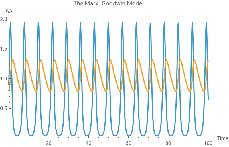
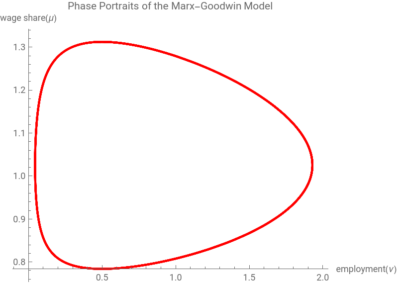
Suppose we have the following arbitrary parameter values and the initial conditions: n = 0.03, σ = 0.15, θ = 0.2, γ = 0.05, and ρ = 0.3, with the initial employment level and labor income share are ν(0) = 10 and μ(0) = 0.8. Then the solution to this system will behave:
In[]:=
ClearAll[n,σ,θ,γ,ρ,μ,ν,t,sol];n=0.03;σ=0.15;θ=0.2;γ=0.05;ρ=0.3;ν0=10;μ0=0.8;sol=NDSolve[{ν'[t](θ-n)ν[t]+((1-μ[t])/σ)ν[t],μ'[t](γ-θ)μ[t]+ρν[t]μ[t],ν[0]0.9,μ[0]0.8},{ν,μ},{t,0,100}]
Out[]=
νInterpolatingFunction,μInterpolatingFunction


In[]:=
Plot[Evaluate[{ν[t],μ[t]}/.sol],{t,0,100},PlotLabel->"The Marx-Goodwin Model",PlotLegends{"employment(ν)","wage share(μ)"},AxesLabel{"Time","ν,μ"},ImageSize->400]
Out[]=


In[]:=
ParametricPlot[Evaluate[{ν[t],μ[t]}/.sol],{t,0,30},PlotLabel->"Phase Portraits of the Marx-Goodwin Model",PlotStyle{Red,Thick},AxesLabel{"employment(ν)","wage share(μ)"},ImageSize->400,AspectRatio->0.8]
Out[]=
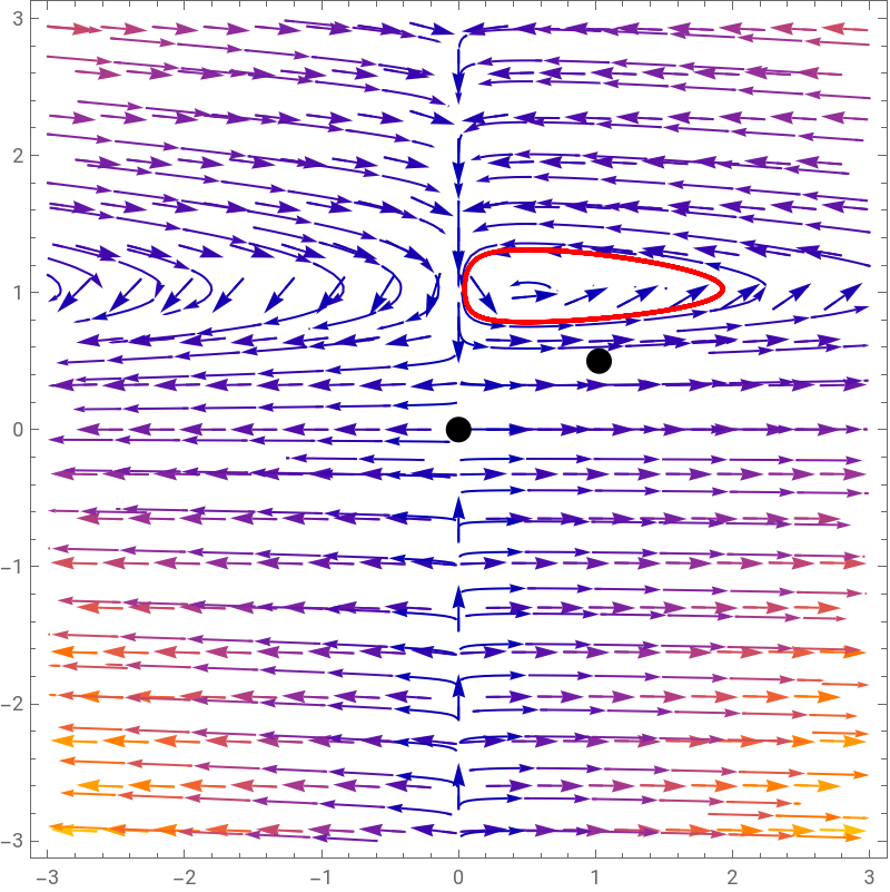
Using both VectorPlot and StreamPlot, we can also visualize the solution inside the vector field as follows:
In[]:=
ShowVectorPlot[{(θ-n)ν+((1-μ)/σ)ν,(γ-θ)μ+ρνμ},{ν,-3,3},{μ,-3,3}],StreamPlot[{(θ-n)ν+((1-μ)/σ)ν,(γ-θ)μ+ρνμ},{ν,-3,3},{μ,-3,3}],ListPlot1-nσ+θσ,,{0,0},PlotStyle{Black,PointSize[0.03]},ParametricPlot[Evaluate[{ν[t],μ[t]}/.sol],{t,0,30},PlotStyle{Red,Thick}],ImageSize->400
-γ+θ
ρ
Out[]=
An interactive visualization of solution curves
An interactive visualization of solution curves
We can also create an interactive chart that shows the dynamic changes of the solution curve with varying parameter values. The following syntax is one ways for doing this job:
In[]:=
ClearAll[n,θ,σ,ρ,γ,ν,μ,ν0,μ0,t,numsol,pp,pxy];GoodwinModel[n_,θ_,σ_,ρ_,γ_][{ν0_,μ0_}]:=Module[{numsol,pp,pxy,vEq,uEq},numsol=NDSolve[{ν'[t]==(θ-n)ν[t]+((1-μ[t])/σ)ν[t],μ'[t]==(γ-θ)μ[t]+ρν[t]μ[t],ν[0]==ν0,μ[0]==μ0},{ν,μ},{t,0,100}];pxy=Plot[Evaluate[{ν[t],μ[t]}/.numsol],{t,0,100},PlotStyle->{{Blue,Thick},{Red,Dashed,Thick}},Frame->True,FrameLabel->{"Time","ν(t),μ(t)"},PlotLabel->"Employment vs. Wage Share over time",GridLines->Automatic,PlotLegends->Placed[{"Employment ν(t)","Wage Share μ(t)"},Bottom],ImageSize->400];pp=Show[StreamPlot[{(θ-n)ν+((1-μ)/σ)ν,(γ-θ)μ+ρνμ},{ν,0,5},{μ,0,5}],ParametricPlot[Evaluate[{ν[t],μ[t]}/.numsol],{t,0,100},PlotStyle->{Red,Thickness[0.005]}],Frame->True,FrameLabel->{"Employment","Wage Share"},PlotLabel->"Phase Portrait: Marx-Goodwin Cycle",PlotRange->{{0,2},{0,2}},GridLines->Automatic,ImageSize->400];GraphicsRow[{pxy,pp},Spacings->20]]Manipulate[GoodwinModel[n,θ,σ,ρ,γ][{ν0,μ0}],Style["Initial Conditions",Bold],{{ν0,0.9,"Initial Employment (ν0)"},0.6,1.5,Appearance->"Labeled"},{{μ0,0.8,"Initial Wage Share (μ0)"},0.5,1.5,Appearance->"Labeled"},Delimiter,Style["Model Parameters",Bold],{{n,0.03,"Labor Supply Growth (n)"},0,0.1,Appearance->"Labeled"},{{θ,0.04,"Productivity Growth (θ)"},0.01,0.1,Appearance->"Labeled"},{{σ,0.15,"Capital-Output Ratio (σ)"},0.1,1,Appearance->"Labeled"},{{ρ,0.2,"Emp. Effect on Wage Share(ρ)"},0.1,0.6,Appearance->"Labeled"},{{γ,0.01,"LM Inst.'s Effect on Wage Share(γ)"},0,0.2,Appearance->"Labeled"},ControlPlacement->Left,SaveDefinitions->True]
Conclusion
Conclusion
We have sought to replicate the Marx-Goodwin business cycle model. The key feature of this model is that the employment rate and wage share (which is 1 minus profit share) interact and behave just as what Lotka-Volterra’s classic predator-prey model shows. The higher profit share speeds up the accumulation of the capital stock, which increases the demand for labor (the employment rate) and the wage share in tandem. This process, in turn, generates a barrier for the continued accumulation of the capital stock. As the accumulation of the capital stock is impeded, the demand for labor and the wage share will fall after a while. This nonlinear dynamic interaction between the employment and profit share repeats itself over time.
One crucial assumption used in Goodwin’s model is that the capital-output ratio and, therefore, the capital-labor ratio remain constant. This assumption is useful for model building purpose, but it is counterfactual in the history of capitalist economic development. Advanced capitalist market economies around the world have shown that there is a strong tendency of rising capital-labor ratio (‘technical/organic composition of capital’ in Marx), which means that fixed capital stock has grown faster than the growth of the demand for labor input. The accumulation of the productive capital stock, in this way, involves a greater increase in non-labor capital equipment relative to the growth of labor input. This aspect of the real-world capitalist development has fundamentally altered the capital-labor relation in many advanced capitalist market economies.
Even with this limitation, however, the Marx-Goodwin model remain a very insightful model for analyzing the dynamic interaction among income share, investment, and employment variable.
Reference
Reference
◼
Hans-Walter Lorenz, Nonlinear dynamical economics and chaotic motion, Berlin: Springer-Verlag, 1989, pp.61-69.
◼
Jorg Glombowski, and Michael Kruger, “A Goodwin cycle with changing regimes of industrial relations,” in P. Flaschel and M. Landesmann (ed.), Mathematical Economics and the Dynamics of Capitalism: Goodwin’s legacy continued, London and New York: Routledge, 2008, Ch. 4.
◼
Karl Marx, Capital - A Critique of Political Economy, Vol. 1, New York and London: Penguin Books, 1990 [1867], Ch 19 and Ch 25.1-25.4.
◼
Richard M. Goodwin, “A growth cycle,” in C. H. Feinstein (ed.), Socialism, Capitalism and Economic Growth, Cambridge: Cambridge University Press, 1975 [1967].
◼
Richard M. Goodwin, Essays in Economic Dynamics, London: Macmillan, 1982 [1971].
◼
Simon Mohun and Robrto Veneziani, “Goodwin cycles and the US Economy, 1948-2004,” in P. Flaschel and M. Landesmann (ed.), Mathematical Economics and the Dynamics of Capitalism: Goodwin’s legacy continued, London and New York: Routledge, 2008, Ch. 6.
CITE THIS NOTEBOOK
CITE THIS NOTEBOOK
Introduction to dynamic economic models: A note on Marx-Goodwin model of business cycles
by Hee-Young Shin
Wolfram Community, STAFF PICKS, January 4, 2026
https://community.wolfram.com/groups/-/m/t/3600562
by Hee-Young Shin
Wolfram Community, STAFF PICKS, January 4, 2026
https://community.wolfram.com/groups/-/m/t/3600562