Explorations in aircraft stability augmented systems: a reinforcement learning approach
by
Carolina Cottas Medeiros
Saulo da Paz Almeida
Greetings! This project is part of the Brazilian Wolfram Conference Hackathon 2021
by
Carolina Cottas Medeiros
Saulo da Paz Almeida
Greetings! This project is part of the Brazilian Wolfram Conference Hackathon 2021
Aircraft SAS
Aircraft SAS
Aircraft automatic control usually brings to mind control architectures for required paths, angles and velocities the airplane needs to maintains during flight. Stability augmentation systems (SAS), in other hand, are control systems in which goal is to avoid dangerous or uncomfortable behavior during maneuvers. They usually bring up the necessity of dealing with the frequencies and damping of the aircraft dynamic modes.
Not only stability
Not only stability
The role of SAS is way beyond placing poles over the right-side of the complex plane. The stability of dynamic modes can’t assure that the pilot actions won’t make the aircraft dive into difficult handling scenarios. For that matter, SAS systems need to attend specific requirements to make it not only safe and stable, but with good handling characteristics.
Exploration
Exploration
The idea behind this project is to explore a simple implementation of a neural network capable of judging the handling qualities of an aircraft longitudinal response to the elevator command, and reallocate its poles to an better condition.
Deep Learning
Deep Learning
The project workflow
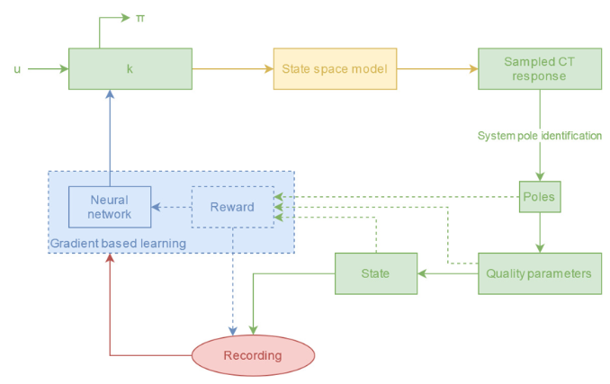
Reinforcement Learning is a method of training a neural network is basically teaching it through trial and error, which means in this case rewarding desired behaviors and punishing undesired ones . This happens by assigning positive values to the desired actions and negative to the undesired ones, making the network seek the maximum overall reward and achieve an optimal solution by avoiding the negative values . By definition, this method is challenging to implement and limited in its application, because it relies on exploration of the environment .
Aircraft Response
Aircraft Response
The longitudinal behaviour of an aircraft can be delivered from a simple implementation over the wolfram’s control systems library . For the model, it was followed a linear-model of an aircraft as shown in [1]. For the parameters, it was used the data given in [1] for a Cessna 310 series. The state-space matrices are given as bellow:
=
x u x Tu | x α U 0 | 0 | -ℊCos[ θ 1 |
U 0 z u U 0 z α | z α U 0 z α | U 0 U 0 z q U 0 z α | - U 0 θ 1 U 0 z α |
M u M Tu | M α M Tα U 0 M α z α U 0 U 0 z α | M α z q U 0 U 0 z α M q | - M α θ 1 U 0 z α |
0 | 0 | 1 | 0 |
ℬ=
x δe |
z δe U 0 z α |
M δe M α z δe U 0 z α |
0 |
As matrice C is an identity matrix and D a zero matrix, in the standard implementation of state-space (SS) models.
In[]:=
(* longitudinal state-space matrixes *) =
;ℬ =
; = IdentityMatrix[4]; =
;
-0.005613748716193086` | 0.004635869907565901` | 0 | -9.7990971` |
-0.020830067014826727` | -0.1678700886854612` | 94.84492029052105` | 0.` |
0.` | -0.005163351659371689` | -0.4097621706964508` | 0.` |
0 | 0 | 1 | 0 |
0.` |
-0.029292281739600086` |
-3.2999077574191444` |
0 |
0 |
0 |
0 |
0 |
Once given the matrices, the model can be explored through:
(* general state-space model *)syslong = StateSpaceModel[{,ℬ,,},SystemsModelLabels{{"δe"},{},{"u","w","q","θ"}}]
Out[]=

| | δe | |||
u | -0.00561375 | 0.00463587 | 0 | -9.7991 | 0. |
w | -0.0208301 | -0.16787 | 94.8449 | 0. | -0.0292923 |
q | 0. | -0.00516335 | -0.409762 | 0. | -3.29991 |
θ | 0 | 0 | 1 | 0 | 0 |
| 1 | 0 | 0 | 0 | 0 |
| 0 | 1 | 0 | 0 | 0 |
| 0 | 0 | 1 | 0 | 0 |
| 0 | 0 | 0 | 1 | 0 |
To have a first look at the model response, let’s check its poles:
TransferFunctionModel[syslong]poles = TransferFunctionPoles[%][[1]]
Out[]=

δe |
- 0.000135795-39963.-227439.s.+ 2 s. 0.00105392+0.00317487s.+0.561844 2 s. 3 s. 4 s. |
- 0.029292322.9946+59.9836s.+10685.1 2 s. 3 s. 0.00105392+0.00317487s.+0.561844 2 s. 3 s. 4 s. |
- 3.299910.00103869s.+0.173438 2 s. 3 s. 0.00105392+0.00317487s.+0.561844 2 s. 3 s. 4 s. |
-0.00342758-0.572329s.-3.29991 2 s. 0.00105392+0.00317487s.+0.561844 2 s. 3 s. 4 s. |
Out[]=
{{-0.289759-0.688356,-0.289759+0.688356,-0.0018644-0.0434278,-0.0018644+0.0434278}}
poles[[1,1]]{Abs@%,Sin[(Abs@Arg@%)-Pi/2]}poles[[1,3]]{Abs@%,Sin[(Abs@Arg@%)-Pi/2]}
Out[]=
-0.289759-0.688356
Out[]=
{0.746856,0.387971}
Out[]=
-0.0018644-0.0434278
Out[]=
{0.0434678,0.0428916}
They both show a stable condition, but very poor handling quality, as we will discuss further along the project. Let’s look at the behaviour of its characteristic equation:
characteristicEquation = 1/(0.0010539219090725605`+0.003174872736349871` s+0.5618437363351814` +0.5832460080981052` +);TransferFunctionModel[k characteristicEquation, s]RootLocusPlot[%,{k,0,5}]RootLocusPlot[%%,{k,0,1},PlotRange{{-.04,.04},{-.06,.06}}]BodePlot[TransferFunctionModel[ characteristicEquation, s]]
2
s
3
s
4
s
Out[]=
k 0.00105392+0.00317487s+0.561844 2 s 3 s 4 s |
Out[]=
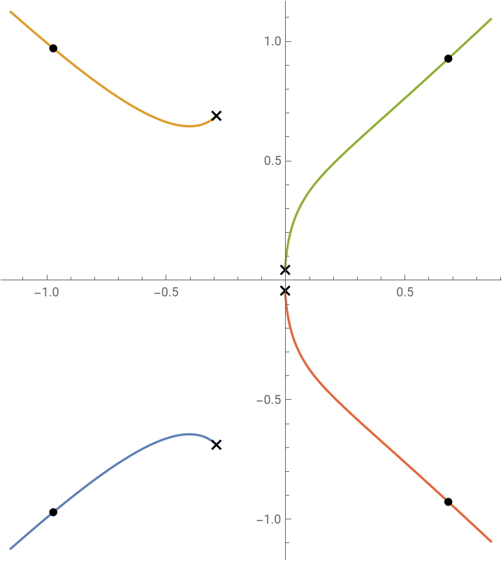
This is a typical behaviour of an aircraft: the two conjugated poles close to the origin determine the mode called phugoid, which is the long term effect over the longitudinal plane; the other two are the short-period mode a “instant-time” (transient effect), for which this project intends to explore over its quality handling.
The Bode-Plots are another confirmation of the usual behaviour of aircraft.
The Bode-Plots are another confirmation of the usual behaviour of aircraft.
Reward System
Reward System
A very well established approach to aircraft handling qualities is given by [4], and for that matter, a set of points was extracted and stated as lists, as follows:
ThumbPrint regions
ThumbPrint regions
For this criteria, the poles of the system corresponding to the short-period mode need to be known, and their natural frequency and damping ratios determined. The ones that fall over the most inner region show ideal behaviour in the pilots’ opinions. The second inner region is satisfactory, the external half-ring show hard to manage and uncomfortable characteristics, and the external area is highly not recommended (the same one where we can locate our “testing plane”). Since the phugoid behaviour lasts longer, it’s easier to deal with and will be accepted as any stable behaviour.
The four regions delimiting the possible results were converted into a function in order to establish a rewarding system which gives a ponctuation of -2, -1, 1, 2 for insatisfatory, poor, acceptable and satisfatory results, respectively.
Furthermore, poles with unstable characteristics are punished in both dynamic modes.
Furthermore, poles with unstable characteristics are punished in both dynamic modes.
Continuous-time model identification
Continuous-time model identification
An algorithm was implemented to identify the system from a sampled data given by the state responses, as proposed by [5]:
Assembling the Environment
Assembling the Environment
System response
A function to sampling the system’s response:
Further implementations
Further implementations
Since the minimal needs to implement were achieved in this time over the Hackathon - we can Observe, act and compute rewards from the system, a implementation of the Deep Learning is close. We couldn’t find a appropriate model for the Brazilian Hackathon delivery of the project, but we have means of creating a dataset to train it.
References
References
[1] Cook, Michael V. Flight dynamics principles: a linear systems approach to aircraft stability and control. Butterworth-Heinemann, 2012.
[2] O’hara, F. “Handling criteria.” The Aeronautical Journal 71.676 (1967): 271-291.
[3] Garnier, Hugues, M. I. C. H. E. L. Mensler, and A. L. A. I. N. Richard. “Continuous-time model identification from sampled data: implementation issues and performance evaluation.” International journal of Control 76.13 (2003): 1337-1357.