CITE THIS NOTEBOOK: Accelerating simulations of systems of particles by Wolfram Emerging Leaders Program. Wolfram Community FEB 17 2023.
The Wolfram Emerging Leaders Program is a 4-month long, project-based program designed for gifted high school students to take a deep dive into a topic of their choice. Students work remotely in small groups to take their project from ideation to completion, with the guidance of Wolfram experts. Wolfram Emerging Leaders Program participants are selected from the Wolfram High School Summer Camp, which is open to talented, STEM-oriented students age 17 and under. This essay was written by:
Simulating how particles interact with each other is a crucial problem that is often addressed using extremely computationally expensive methods. We propose a hybrid Transformer based neural network that attempts to predict the next state of a system, achieving a significant speedup over classical methods.
Accelerating Simulations of Systems of Particles using a Transformer based Machine Learning Architecture
Accelerating Simulations of Systems of Particles using a Transformer based Machine Learning Architecture
Motivation
Current particle simulations are slow and difficult to parallelize, limiting their use by individuals or organisations with high computational resources. Our work is concerned with distilling the knowledge of a system’s behaviour from a traditional simulation method (such as EPOCH) into a Machine Learning system that is easily parallelized and has good inference performance, although potentially more difficult to train on consumer hardware.
Methodology
Given the high complexity of the environments we wanted to simulate, we decided to simplify the problem: First, we decided to work in a 1d setting, and second, we divided the environment into a grid-like structure and calculated the densities of the particles in each of these regions. Then we worked on predicting which distribution of particle densities would emerge next.
Our initial approach used a Convolutional Autoencoder to learn the features and a Recurrent Neural Network (RNN) to predict subsequent states, but we eventually switched to a plain Transformer-based architecture. A Convolutional Autoencoder is a type of neural network particularly suited to learning features from data that can be represented as a grid, such as images. It works by encoding the input into a lower dimensional representation and then decoding it back into its original space. This process causes the Autoencoder to learn important aspects of the data that can be used for a variety of tasks.
In order to train our machine learning model, we needed to collect a dataset to use as training data. We obtained such data by running a series of simulations with a state-of-the-art physics engine that simulates the evolution of a system over time. These simulations were run for different conditions, such as different initial densities.
After creating the simulation dataset, we pre-processed it by normalising and dividing it into training and test. We then used this data to train our machine learning model.
Data collection
To collect the data, we used a code called EPOCH, which is a Particle in Cell (PIC) simulation code. Particle in Cell is a molecular dynamics simulation method that uses explicit particles, such as individual electrons and nuclei, to generate electric and magnetic fields on a lattice, and uses these to calculate the forces and motions of pseudo-particles, which are groups of smaller particles. The simulation we ran consisted of two streams of electrons moving in opposite directions, confined in a one-dimensional environment, similar to a particle collider. We ran our simulations on an Ubuntu GNU/Linux machine.
The electron Two-Stream Instability
The two-stream electron instability is a hypothetical situation in which two electron beams travelling in opposite directions collide. The charges on the electrons cause changes in the electric fields, which in turn affect the speed of the travelling electrons and the density of the combined streams at each point.
Data loading
Data loading
NOTE: To run the Notebook you must first download the data.
NOTE: Bear in mind that the data used in this Notebook has gone through Feature Scaling to ease training.
data=Import["path/to/data"];
Autoencoder dataset preprocessing
Autoencoder dataset preprocessing
In[]:=
autoencoderDataset=Join@@Table[(#->#)&/@episode,{episode,data}]
We divide the data into train and test for evaluation purposes.
In[]:=
{trainAutoencoderDataset,testAutoencoderDataset}=ResourceFunction["TrainTestSplit"][autoencoderDataset,"TrainingSetSize"->Scaled[0.95]]
Original Architecture
Original Architecture
Our original architecture employed a based architecture which operates on a Latent Space learned by a Convolutional but we eventually decided to switch over a plain Decoder-Only Transformer. We later repurposed the Convolutional Autoencoder to work as a metric to evaluate our main prediction model.
Transformer
Autoencoder
Autoencoder
Autoencoder
The is composed of an Encoder and a Decoder. The goal of this model is to reconstruct the input by forcing the data to pass into a bottleneck, thus learning a lower dimensional representation.
Autoencoder
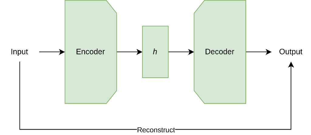
For modularity reasons, the whole architecture is split in small pieces, the Blocks, that we then put together.
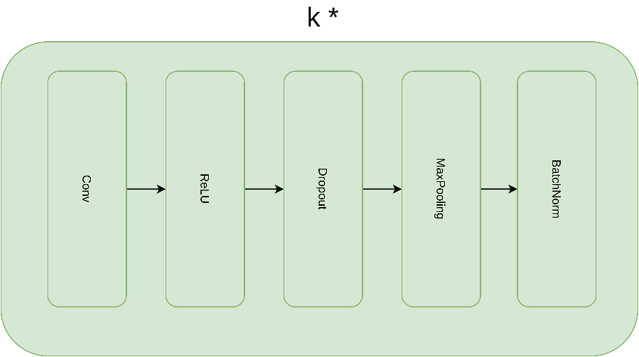
The convPoolBlock has the purpose of applying the convolution operation and then reduce the size of the feature map.
In[]:=
convPoolBlock[num0_Integer,dropoutRate0_?NumberQ,stride0_Integer:2]:=Module[{num=num0,dropoutRate=dropoutRate0,stride=stride0},(NetChain[{ConvolutionLayer[num,{3},PaddingSize->1],Ramp,DropoutLayer[dropoutRate],PoolingLayer[{2},stride,"Function"->Max],BatchNormalizationLayer[]}])]
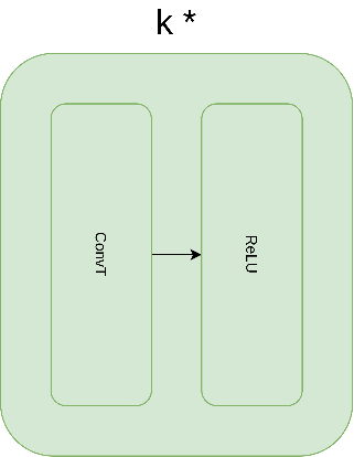
The convTBlock executes a transposed convolution operation, increasing the size of the feature map, this is used in the data reconstruction phase.
In[]:=
convTBlock[num0_Integer,stride0_Integer:2]:=Module[{num=num0,stride=stride0},(NetChain[{DeconvolutionLayer[num,{2},"Stride"->stride],Ramp}])]
In[]:=
gridSize=400;
In[]:=
autoencoderDropoutRate=0.44;
We advice to run the training on a GPU.
In[]:=
device="GPU";
The Encoder is composed of k equal Encoder Blocks, which are Convolution operations followed by Batch Normalization.
The Encoder uses a kernel size of 3 and 2 for pooling, we’ve found empirically that those hyperparameters give the best results on our task.
In[]:=
autoencoderEncoder=NetChain[{ReshapeLayer[{1,gridSize}],convPoolBlock[32,autoencoderDropoutRate],convPoolBlock[16,autoencoderDropoutRate],convPoolBlock[8,autoencoderDropoutRate],convPoolBlock[8,autoencoderDropoutRate]}]
Out[]=
NetChain


The Decoder is composed of k equal Decoder Blocks, which are Convolution operations.
In[]:=
autoencoderDecoder=NetChain[{convTBlock[8],convTBlock[8],convTBlock[16],convTBlock[32],ConvolutionLayer[1,{1}],FlattenLayer[]}]
We proceed with the training of the the Autoencoder.
The following plot represents the Hidden Representation that the model has of the system.
The following plot represents the distribution of particles over space.
The sequences are encoded in the Latent Space, this allows us to understand how different states relate to each other, this is also especially useful for clustering.
Predictor dataset preprocessing
Predictor dataset preprocessing
We divide the data into train and test for evaluation purposes.
Transformer
Transformer
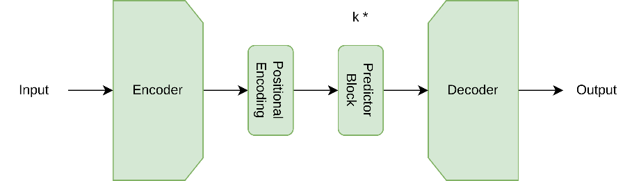
We make use of a Decoder-Only Transformer architecture, the model takes in input a sequence of past states of the system and tries to predict the next.
The Positional Encoding is used by the model to allow the Attention Mechanism to take in consideration the position of the system states in time, in our model, we implement a Learned form of Positional Encoding, which means that we learn an embedding for each position in the sentence which is then added to each element.
The pointwiseBlock is a Feed-Forward Neural Network which operates on the hidden embeddings of the Transformer, this part is actually responsible for learning the task of prediction.
Our predictor uses 6 heads, which means that attention is calculated 6 times in parallel, giving the model a more complete view for each state.
Self-Attention works by calculating the correlations between each item in the sequence and all the others, so that it can identify items that contain useful information. This allows the model to take into account previous elements to make a more informed prediction.
The Decoder Block is at the core of the Transformer, it processes the Hidden Embeddings and applies the Self-Attention Mechanism, then, it applies a Feed Forward Neural Network that "transforms" the embeddings to then be processed again.
The Classification Head is responsible for taking the output embeddings from the model and computing the actual predictions from them, in other words, in turns data from the "meaning space", to the "system space".
During training, we shift the goals by 1 so that the model learns to map each state of the system to the next, taking into account only
the previous observations.
the previous observations.
We proceed with the training of the the Transformer.
The following plot represents the distribution of particles over space.
Evaluation
We use our Convolutional Autoencoder to measure the distance of the latent of the predicted system state from the actual, which we use as our metric.
The points are mostly grouped in clusters of 2, this means that predicted states are similar to the actual.
Knowing where the predictions and actuals lie in the embedding space, we can calculate the average distance between them and use it as a metric.
Performances
Because the Neural Network doesn’t have to deal with each individual particle, it is able to compute a prediction much faster than traditional methods, unfortunately a direct comparison with EPOCH is not possible due to the fact that the latter was developed to work on CPUs only, whereas Neural Networks perform much better on GPUs, benefiting greatly from the Accelerated Computing paradigm.
It’s important to note that this result was obtained on a consumer GPU (RTX 3060 Ti) and is likely to improve on more powerful hardware.
Possible future developments
Due to computational limitations, our system is currently trained on a small pool of data; It has been shown that increasing both the model size and the amount of data tends to dramatically improve the results.
Glossary
1
.Encoder. A model that maps some data from a high dimension to a lower one.
2
.Decoder. A model that maps some data from a low dimension to a higher one.
3
.Autoencoder. A model that (in most scenarios) tries to reconstruct its input by making data pass through a bottleneck. It’s composed of an Encoder and a Decoder.
4
.Neural Network. A Neural Network is a type of machine learning system which operates using an approximate model of a neuron.
5
.Recurrent Neural Network. Also known as an RNN, it’s a particular class of Neural Network which is well suited to work on sequential data.
6
.ReLU. Short for Rectified Linear Unit, a non-linearity function often used in Neural Networks.
7
.Convolutional Neural Network. Also known as CNN, it’s a particular class of Neural Network that deals with spatial data.
8
.Pooling. An operations mostly used in Convolutional Neural Networks (CNNs) to reduce the dimension of the features map.
9
.Overfitting. A phenomenon that verifies whenever a model too closely approximates the training dataset failing to generalize.
10
.Dropout. A technique that randomly “kills” a percentage of a Neural Network’s layer at training time in order to prevent overfitting.
11
.Batchnorm. Short for Batch Normalization, it’s a technique used to increase the efficiency of the training of Neural Networks.
12
.Positional Encoding. A function that takes in input a sequence of embeddings and encodes positional information.
13
.Self-Attention. A mechanism that allows a model to create relations between elements in a sequence.
14
.Transformer. A model architecture that is well suited with working on sequential data.
Citations
1
.Autoencoder. Rumelhart et al. 1986.
2
.Transformer. Vaswani et al. 2017.
3
.EPOCH. EPOCH contributors.
4
.PIC. Hockney, Eastwood 1988.