ABSTRACT: A new Wolfram resource function has been developed to solve a specific class of nonlinear integral equations, known as the Thermodynamic Bethe Ansatz (TBA). These equations have been extensively studied in theoretical physics over recent decades, with applications ranging from statistical mechanics to gauge and string theory. Due to their very involved form, TBA equations cannot be tackled using the DSolve superfunction and require a special numerical framework. CITATION (original articles): D. Fioravanti, D. Gregori (2020), Integrability and cycles of deformed N=2 gauge theory, Physics Letters B, Volume 804. https://doi.org/10.1016/j.physletb.2020.135376
D. Fioravanti, D. Gregori and H. Shu (2022), Integrability, susy SU(2) matter gauge theories and black holes, arXiv:2208.14031. https://doi.org/10.48550/arXiv.2208.14031
D. Fioravanti, D. Gregori and H. Shu (2022), Integrability, susy SU(2) matter gauge theories and black holes, arXiv:2208.14031. https://doi.org/10.48550/arXiv.2208.14031
Author Writing
Author Writing
Introduction
Introduction
Most applied mathematics has been developed in terms of the so-called “differential equations”. These are relations which involve an unknown function and its derivatives [a]. Much less widely used is another type of relations: the so-called “integral equations”. They involve the operation inverse to the derivative, which is the integral. As is well known, integrals are generally much more difficult to compute than derivatives and arguably it is for this reason that solving integral equations has not become common practice.
Also the software world is still quite devoid of good packages and frameworks for solving integral equations. Mathematica for example can solve symbolically some simple integral equations through the functionality (the same tool that solves differential equations), but it has no way to solve more complex integral equations ( does not apply). For these, numerical integral equation algorithms would be required because, by weakening the requirement for a symbolic solution - that is, accepting even just numerically interpolated solutions - the range of solvable integral equations would vastly increase.
ThermodynamicBetheAnsatzSolve
ThermodynamicBetheAnsatzSolve
Thus, I am happy to announce that I have started to change this scenario by developing the first Wolfram resource function to solve numerically a particular type of integral equations: the Thermodynamic Bethe Ansatz (TBA).
These integral equations take the following general form:
y
j
f
j
n
∑
k1
∞
∫
-∞
φ
j,k
c
j,k
σ
j,k
y
k
where (x) , for are the dependent variables, (x) the non-homogeneous (or forcing) terms, (x) the integral kernels, some constants and ±1. Notice that the integral terms are always convolutions and the equation is highly nonlinear.
y
j
j1,…,n
f
j
φ
j,k
c
j,k
σ
j,k
If you are interested in knowing more about the theoretical physics applications of this type of equations, read below a LLM-assisted review of the main arXiv papers on that.
In my former research, I often needed to solve TBA equations [b]. However, the code I initially learned from my colleagues worked for only particular instances of TBA equations and each time required a lot of redundant and painful manual recoding (besides having several other disadvantages). Instead the new resource function only requires the user to specify the TBA equation and then it fully automatically and rapidly delivers its solution.
Code Examples
Code Examples
Sinh-Gordon TBA
Sinh-Gordon TBA
For instance, solve the TBA for the Sinh-Gordon integrable model:
In[]:=
tbaSHG=y[x]rCosh[x]-t;
∞
∫
-∞
Log[1+]Sech[t-x]
-y[t]
2π
In[]:=
ResourceFunction["ThermodynamicBetheAnsatzSolve"][tbaSHG/.r->0.1]
Out[]=
yInterpolatingFunction


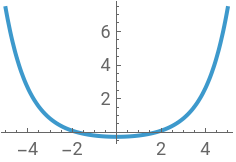
This yields a solution in the form of an interpolating function, which can be visualized as follows:
In[]:=
Plot[y[x]/.%,{x,-5,5}]
Out[]=
AdS/CFT TBA
AdS/CFT TBA
A more interesting example is the following “monstrous” system of hundreds (in principle, an infinity) of TBA equations:
In[]:=
χ[a_,x_]:=ψ[a_,x_]:=ϕ[a_,x_]:=tbaFFPT[p_]:=tbaFFPT[p]=Block{A},A[_,i_,j_]:=KroneckerDelta[i,j+1]+KroneckerDelta[i,j-1];Union@Joiny0[x]==mRCosh[x]+Iα-Sumχ[1-2l/4,x-t]Log[1+Exp[Symbol["y"<>ToString@l<>"a1"][t]]]t,{l,1,3}-Sumψ[1-2l/4,x-t]Log[1+Exp[Symbol["y"<>ToString@l<>"a1"][t]]]t,{l,1,3},y0b[x]==mRCosh[x]-Iα-Sumχ[1-2l/4,x-t]Log[1+Exp[Symbol["y"<>ToString@l<>"a1"][t]]]t,{l,1,3}+Sumψ[1-2l/4,x-t]Log[1+Exp[Symbol["y"<>ToString@l<>"a1"][t]]]t,{l,1,3},Flatten@TableSymbol["y"<>ToString[i]<>"a"<>ToString[j]][x]==KroneckerDelta[i,1]KroneckerDelta[j,1]ϕ[2,x-t]Log[1+Exp[-y0[t]]]t+KroneckerDelta[i,3]KroneckerDelta[j,1]ϕ[2,x-t]Log[1+Exp[-y0b[t]]]t+SumA[∞,l,j]ϕ[2,x-t]Log[1+Exp[Symbol["y"<>ToString@i<>"a"<>ToString@l][t]]]t,{l,1,p-1}-SumA[3,l,i]ϕ[2,x-t]Log[1+Exp[-Symbol["y"<>ToString@l<>"a"<>ToString@j][t]]]t,{l,1,3},{i,1,3},{j,1,p-1};
2
π
CosCosh[x]
aπ
2
Cos[aπ]+Cosh[2x]
1
π
Sin[aπ]
Cos[aπ]+Cosh[2x]
1
2π
a
Cosh[ax]
1
2
K
∫
-K
1
2
K
∫
-K
1
2
K
∫
-K
1
2
K
∫
-K
K
∫
-K
K
∫
-K
K
∫
-K
K
∫
-K
For example, with parameter , the TBA consists of 29 coupled equations:
p=10
In[]:=
tbaFFPT[10]//TabView
Out[]=
Remarkably, after just a few hours of study, with my resource function I was able to reproduce the results of a string theory paper [1]:
In[]:=
centralCharge[p_,mm_,RR_,αα_,KK_:20,options:OptionsPattern[]]:=Block{sol},sol=ResourceFunction["ThermodynamicBetheAnsatzSolve"][tbaFFPT[p]/.{m->mm,R->RR,K->KK,α->αα},options];3mmRRπ^2NIntegrateCosh[t]Log[1+]+Log[1+]/.sol,{t,-KK,KK}[[1]]centralChargeLimit[p_]:=p(1-p-4+4^2+2*4p)/(4+p)/(3+p)//N
-y0[t]
-y0b[t]
(*Warning:thefollowingcomputationtakesalongtimeandcanstressyourcomputer!*)
In[]:=
ParallelTable[{p,centralChargeLimit[p],centralCharge[p,1*10^(-17),1*10^(-17),0,600,"GridResolution"->2^14,"SaveMemory"->True]//Quiet},{p,2,41,3}]//Prepend[#,{"p","cent. charge (analytic)","cent. charge (TBA)"}]&//TableForm
Out[]//TableForm=
p | cent. charge (analytic) | cent. charge (TBA) |
2 | 1.8 | 1.8 |
5 | 3.33333 | 3.33333 |
8 | 4.18182 | 4.18182 |
11 | 4.71429 | 4.71429 |
14 | 5.07843 | 5.07843 |
17 | 5.34286 | 5.34286 |
20 | 5.54348 | 5.54348 |
23 | 5.70085 | 5.70086 |
26 | 5.82759 | 5.82759 |
29 | 5.93182 | 5.93182 |
32 | 6.01905 | 6.01905 |
35 | 6.09312 | 6.09312 |
38 | 6.15679 | 6.1568 |
41 | 6.21212 | 6.21212 |
Final Thoughts
Final Thoughts
A final reflection is due. TBA equations have been thoroughly studied by mathematical physicists for more than 30 years. However, this Wolfram resource function seems the only actual package thus far (on GitHub, there exists only sparse code for very special equations). One should then wonder: why has nobody else come up with an open package to solve TBA equations before?
The reason, unfortunately, is pretty clear. The fact is that in the academic system, well-written software is valued much less than apparently rigorous peer-reviewed papers. (By the way, Wolfram Research also reviews resource functions and I often find it very helpful and instructive.) Besides, academics naturally take advantage of being obscure to their colleagues, who otherwise could do the same computations and publish the same papers. The greatest problem with this professional dynamic is that, if not properly curated and published, the code underlying the supposed academic “progress” is likely to become lost forever [c].
LLM Writing
LLM Writing
ArXivExplore install
ArXivExplore install
In[]:=
PacletInstall["DanieleGregori/ArXivExplore"]
Out[]=
PacletObject
In[]:=
Needs["DanieleGregori`ArXivExplore`"]
Find TBA titles
Find TBA titles
In[]:=
tbaIdsOfTitles=Keys@ArXivLogosTitles[Or["thermodynamic bethe","tba"],{"hep-th",All}];tbaAbstractsToIds=AssociationMap[Reverse,AssociationMap[ArXivAbstracts[#]&,tbaIdsOfTitles]];
TBA abstracts SemanticRanking
TBA abstracts SemanticRanking
In[]:=
extractor=NetModel["SciBERT Trained on Semantic Scholar Data"];reranker=Function[{reference,candidates},EuclideanDistance[Mean[#],Mean[extractor[reference]]]&/@extractor[candidates]];
In[]:=
tbaAbstractsRanked=SemanticRanking[Keys[tbaAbstractsToIds],"Thermodynamic Bethe Ansatz, TBA",Method->reranker];
In[]:=
tbaRefs=Lookup[tbaAbstractsToIds,Take[tbaAbstractsRanked,20]];
ArXivExplain TBA
ArXivExplain TBA
In[]:=
tbaExplanation=ArXivExplainConcept["Thermodynamic Bethe Ansatz (TBA)",tbaRefs]//Quiet
Out[]=
The Thermodynamic Bethe Ansatz (TBA) is a powerful method developed for studying the thermodynamics of integrable quantum field theories, especially in one-dimensional systems. It emerged as a means to compute the ground state energy and finite temperature properties of models described by Bethe ansatz solutions. The core principles of TBA revolve around the interplay between the statistical mechanics of a many-body system and the integrability of the underlying model.### Key Features of TBA:1. **Connection to Bethe Ansatz**: The TBA approach stems from the Bethe Ansatz, which is an exact method for finding the eigenvalues and eigenstates of integrable models. The Bethe Ansatz provides a way to express the wave functions of a system of particles in terms of a set of rapidity variables.2. **Thermodynamic Limit**: TBA is particularly useful in the thermodynamic limit, where the number of particles goes to infinity. In this limit, one can construct a grand canonical ensemble by allowing for the occupation of states defined by the Bethe Ansatz.3. **Energy Density and Free Energy**: The main goal of TBA is to find expressions for the energy density and free energy of the system. This is done through the introduction of Y-functions, which encode the distribution of particles in the system.4. **Integral Equations**: TBA typically leads to a set of non-linear integral equations for these Y-functions. These equations express the relationship between the Y-functions of different particle types and their distribution in the thermodynamic ensemble.5. **Asymptotic Analysis**: In many cases, TBA equations can be solved asymptotically, providing insights into the scaling behavior of the system. This analysis can yield valuable information about phase transitions, correlation lengths, and critical exponents.6. **Correlation Functions**: TBA also enables the computation of correlation functions in integrable models, linking the energy spectrum to physical observables in the system.### Application Across Fields:TBA has found applications in various domains, particularly in high-energy theoretical physics (such as string theory and gauge theories) and statistical mechanics (such as spin chains and percolation models). It plays a crucial role in the AdS/CFT correspondence, which relates string theory in anti-de Sitter space to conformal field theories.### Conclusion:The Thermodynamic Bethe Ansatz is an elegant framework that leverages the structure of integrable models to study the thermodynamic properties of quantum systems. Despite its roots in one-dimensional physics, its implications reach far into various fields of theoretical physics, illustrating the intricate connections between exactly solvable models, statistical mechanics, and quantum field theory.
Notes
Notes
Author Notes
Author Notes
LLM Notes
LLM Notes
References
References
Author References
Author References
LLM References
LLM References
CITE THIS NOTEBOOK
CITE THIS NOTEBOOK
Resource function for the numerical solution of certain nonlinear integral equations
by Daniele Gregori
Wolfram Community, STAFF PICKS, September 23, 2025
https://community.wolfram.com/groups/-/m/t/3549711
by Daniele Gregori
Wolfram Community, STAFF PICKS, September 23, 2025
https://community.wolfram.com/groups/-/m/t/3549711