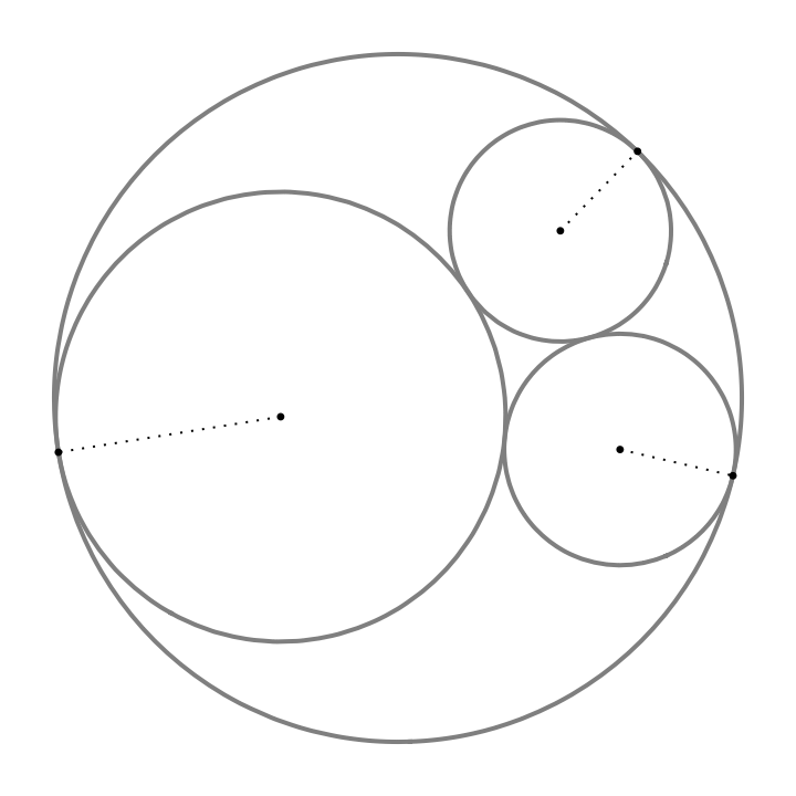
We draw Soddy circles directly, which are the building blocks of the Apollonius gasket. As explained in various articles, when three circles are tangent to each other, we can find a larger circle (or a smaller circle between them) that circumscribes them. Here, we will explore a direct method to create the second and third circles when the first circle is placed inside the larger circle.Problem Statement: Suppose that we have a large circle with radius centered at the origin. Also suppose that we know the center of the first circle inside the large circle, in polar coordinates. To draw a second circle inside, which is tangent to both the circumcircle and the first circle, we only need , the polar angle of the center of the second circle. That is, we cannot draw the second circle with arbitrary values of the radius and . The radial length is determined automatically. The location of the third circle, should be determined automatically as well. Here we derive explicit formulas for , , and .As described above, suppose that we have the radius r0 and the center of the first inner circle (r1, at1). Then the tangent point of the first inner circle (p1Tx, p1Ty) to the circumcircle is automatically given as follows. Furthermore, let's assume we are provided with at2, the polar angle of the second circle. r1T is the radius of the first circle.
r
0
(,)
r
1
θ
1
θ
2
r
2
θ
2
r
2
(,)
r
3
θ
3
r
2
r
3
θ
3
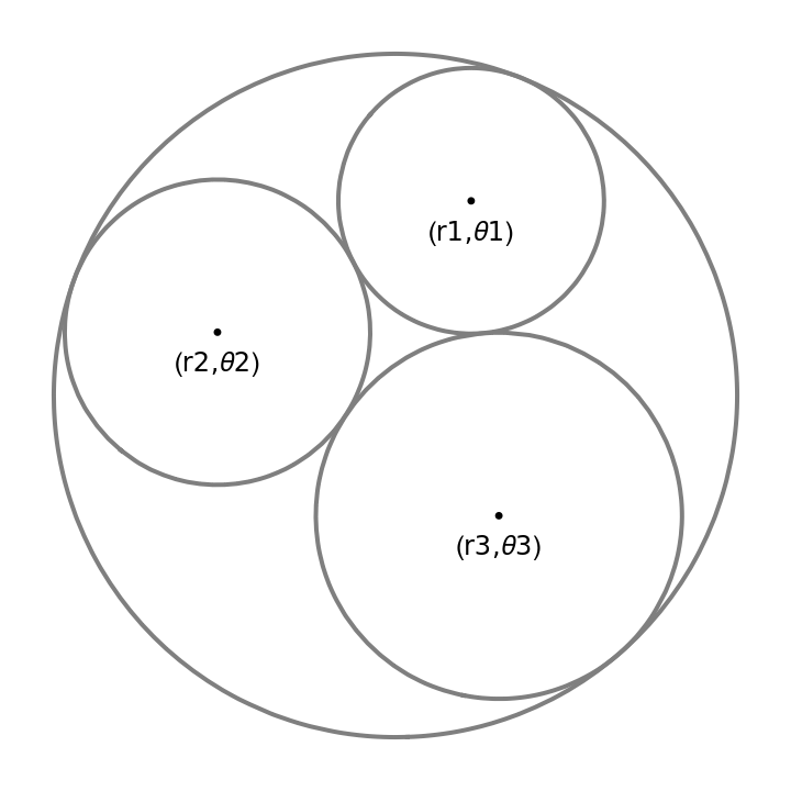
θ
2
In[]:=
ClearAll["Global`*"];p1={p1x,p1y}={r1*Cos[at1],r1*Sin[at1]};p1T={p1Tx,p1Ty}={r0*Cos[at1],r0*Sin[at1]};r1T=r0-r1;p2T={p2Tx,p2Ty}={r0*Cos[at2],r0*Sin[at2]};
Next, we calculate the Cartesian coordinates (p2x, p2y) of the center of the second circle. These coordinates correspond to the polar coordinates (r1, at2), which is equivalent to finding the value of r1 or r2T, the radius of the second circle. To find p2x, we need to solve the equation
(*p2y=Tan[at2]*p2x;r2T=Sqrt[(p2x-p2Tx)^2+(p2y-p2Ty)^2];d12=Sqrt[(p1x-p2x)^2+(p1y-p2y)^2];d12r1T+r2T;Solve[%,p2x]*)
In practice, this code was not executed directly; rather, the calculation was performed by squaring both sides of the equation d12 == r1T + r2T to simplify the process for Mathematica to execute. Consequently, we arrive at the following explicit formulas:
In[]:=
p2x=(2r0(r0-r1)Cos[at2])/(2r0-r1-r1Cos[at1-at2]);p2y=Tan[at2]*p2x;p2={p2x,p2y};d12=(2r0^2-2r0r1+r1^2-r1(2r0-r1)Cos[at1-at2])/(2r0-r1-r1Cos[at1-at2]);r2T=d12-r1T;
Now let's determine the coordinates (r3, at3) of the third circle, as explained earlier. To achieve this, if the radius r3T of the third circle is defined by a formula, and the coordinates of the point where the third circle touches the circumcircle are given as (p3Tx, p3Ty), the following conditions must be satisfied:
In[]:=
p3T={p3Tx,p3Ty}={r0*Cos[at3],r0*Sin[at3]};r3T=Sqrt[(p3x-p3Tx)^2+(p3y-p3Ty)^2];d23=Sqrt[(p2x-p3x)^2+(p2y-p3y)^2];d31=Sqrt[(p3x-p1x)^2+(p3y-p1y)^2];(*Solve[{d23r2T+r3T,d31r1T+r3T},{p3x,at3}]*)
Subsequently, we get two independent equations, d23r2T+r3T and d31r1T+r3T. By solving these together, we must get p3x and at3. Indeed, the calculation was carried out by converting these into a format that Mathematica can interpret. As a result, we deduce the following explicit formula.
In[]:=
nsVal=2r1^2(-2r0^2+4r0r1+r1^2)Cos[at1]+r1^2((4r0^2-8r0r1+5r1^2)Cos[at1-2at2]+r1^2Cos[3at1-2at2]+4r0(r0-2r1)Cos[2at1-at2])+4(4r0^4-16r0^3r1+23r0^2r1^2-14r0r1^3+2r1^4)Cos[at2];sqVal=8(r0-r1)r1Sin[(at1-at2)/2]^2(4r0^2Sin[at2]+r1(-8r0Sin[at2]+r1(-2Sin[at1]+Sin[2at1-at2]+5Sin[at2])));deVal=(2(8r0^4-32r0^3r1+52r0^2r1^2-40r0r1^3+15r1^4-4r1^2(2r0^2-4r0r1+3r1^2)Cos[at1-at2]+r1^2(4r0^2-8r0r1+5r1^2)Cos[2(at1-at2)]));at3a=-ArcCos[(nsVal-sqVal)/deVal];at3b=ArcCos[(nsVal-sqVal)/deVal];at3c=-ArcCos[(nsVal+sqVal)/deVal];at3d=ArcCos[(nsVal+sqVal)/deVal];p3x=(2r0(r0-r1)Cos[at3])/(2r0-r1-r1Cos[at1-at3]);p3y=Tan[at3]*p3x;p3={p3x,p3y};
Note that at3 has four solutions: ±ArcCos[(nsVal ± sqVal)/deVal]. We have omitted careful consideration of the conditions for the range of each polar angle and similar factors, so some of these at3 results might not accurately depict the position of the third inner circle. For practical visualization purposes, these results should suffice. With this, all the necessary components are in place. The actual plotting can be done as shown below:
In[]:=
(*OutputFormatting*)nRad=1;lAxesOptions={AspectRatioAutomatic,TicksNone,AxesOrigin{0,0},PlotRange{{-100,100},{-100,100}},AxesFalse,FrameFalse};(*InitialData*)at3=at3a;r0=90;r1=55;at1=1.2;at2=2.8;(*Drawing*)d1=Graphics[{Black,Disk[p1,nRad]}];d2=Graphics[{Black,Disk[p2,nRad]}];d3=Graphics[{Black,Disk[p3,nRad]}];d1T=Graphics[{Black,Disk[p1T,nRad]}];d2T=Graphics[{Black,Disk[p2T,nRad]}];d3T=Graphics[{Black,Disk[p3T,nRad]}];lP1=Graphics[{Dotted,Black,Line[{p1,p1T}]}];lP2=Graphics[{Dotted,Black,Line[{p2,p2T}]}];lP3=Graphics[{Dotted,Black,Line[{p3,p3T}]}];g0=ContourPlot[x^2+y^2==r0^2,{x,-r0,r0},{y,-r0,r0},ContourStyleGray];g1=ContourPlot[(x-p1x)^2+(y-p1y)^2==r1T^2,{x,-r0,r0},{y,-r0,r0},ContourStyleGray];g2=ContourPlot[(x-p2x)^2+(y-p2y)^2==r2T^2,{x,-r0,r0},{y,-r0,r0},ContourStyleGray];g3=ContourPlot[(x-p3x)^2+(y-p3y)^2==r3T^2,{x,-r0,r0},{y,-r0,r0},ContourStyleGray];Show[g0,g1,g2,g3,lP1,lP2,lP3,d1,d2,d3,d1T,d2T,d3T,lAxesOptions]
Out[]=
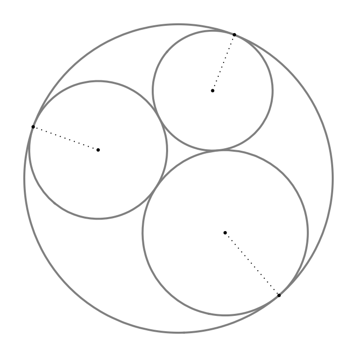
For r1 = 61, at1 = 0.8, at2 = 3.3, the ouput is: