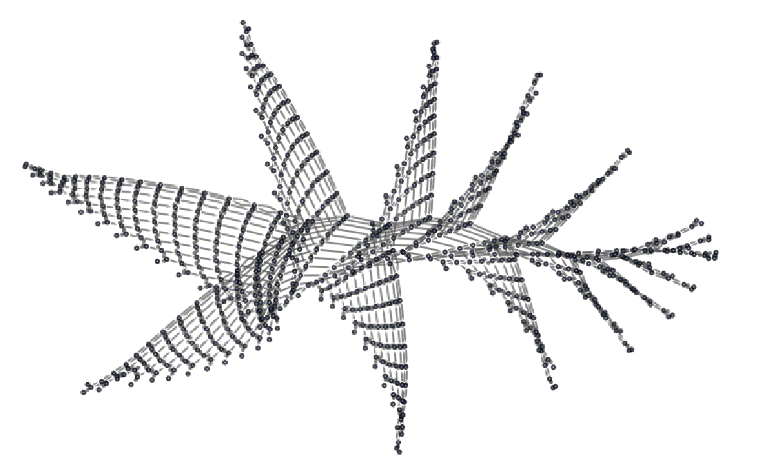
Motivation
Motivation
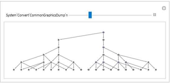
This project focuses on two features of a string substitution multiway system: the phenomenon of termination and the effects of performing completion procedures. The former occurs when a system’s rules do not apply to the latest states anymore (which could have interesting implications to using the Wolfram Models to describe spacetime singularities, see ). Try manipulating a system which is designed to totally terminate at step 15! The object below is the structure of a “multiway state graph” at step number n of its evolution.
In[]:=
Manipulate[ResourceFunction["MultiwaySystem"][{"A""BB","B""CC","C""DD","D"""},"A",n,"StatesGraphStructure"],{n,0,20,1},SaveDefinitionsTrue]
Out[]=
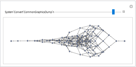
Or this one (terminates to an empty string at step 18):
In[]:=
Manipulate[ResourceFunction["MultiwaySystem"][{"A""B","A""C","C""DD","D""EE","E""XX","X""","B""FF","F""GG","G""YY","Y"""},"A",n,"StatesGraphStructure"],{n,0,20,1},SaveDefinitionsTrue]
Out[]=
The latter feature (completion procedures) is a method which is theorized to be relevant to a quantum observer making measurements, effectively creating their own perception of time by forcing many paths of evolution to converge to a single thread of causal relationships (see ) . We hope to gain knowledge of what proportions of these nondeterministic computational systems behave on terminating ways, as well as to discover interesting behaviors which might eventually be helpful to formulating a “multiway quantum theory”. Try seeing the effects of completion procedures by watching this completed system grow, where the red vertices belong to the original system while the blue ones correspond to new states added by a completion procedure!
In[]:=
CompletionEffects[rules_,init_]:=Manipulate[HighlightGraph[ResourceFunction["MultiwaySystem"][Join[rules,ResourceFunction["MultiwaySystem"][rules,"CanonicalKnuthBendixCompletion"]],init,n,"StatesGraphStructure"],VertexList[ResourceFunction["MultiwaySystem"][rules,init,n,"StatesGraphStructure"]]],{n,0,10,1}]
In[]:=
CompletionEffects[{"A""B","A""C","B""BB","C""CC"},"A"]
Out[]=
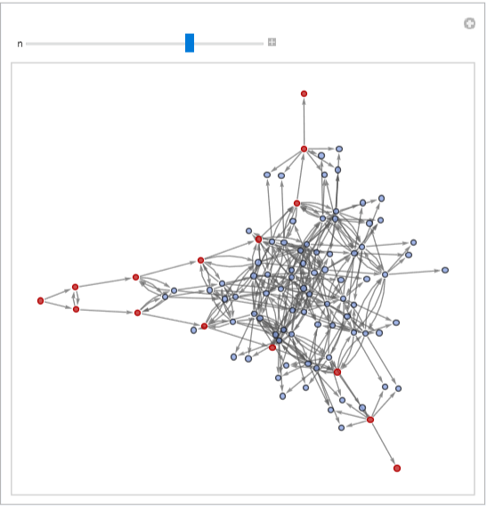
While this one generates subgraphs which grow into isomorphic structures at each step (Warning: higher step numbers give prettier graphs but they might break you laptop):
In[]:=
CompletionEffects[{"AB""A","AA""BAA"},"AAAA"]
Out[]=


Introduction
Introduction
String substitution systems are likely one of the simplest multiway systems. We are given a string and a set of rules describing how its substrings are to be replaced by other substrings, and that is all the information needed to describe the initial state of such a system. For instance, we might start with the state “A”. With rules specifying that each “A” gets replaced by either “AB” or “BA”, we get a system which evolves like this:
Out[]=
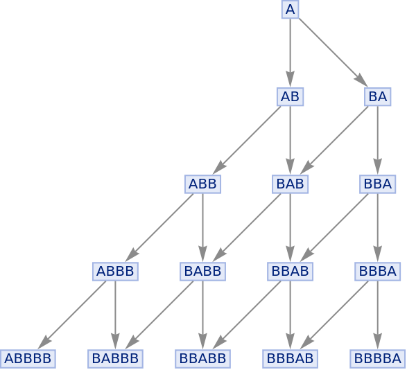
This state graph has strings as vertices, and each directed edge corresponds to a potential application of some rule which “reduces” a string to another. A string can also be interpreted as a combination of distinguishable “colors”, that is: the above system, {AAB, ABA}, is in every way equivalent to something like this: , as long as we change the specification of initial states accordingly. Just like an abundance of simple systems exhibiting complex behaviors, the string substitution system is deceptively simple to describe. Similar to a proper Wolfram Model, which is a graph that evolves by changing its local structures, a string substitution system may evolve in various ways depending on the order and location each rule is applied. If a rule may be applied to different parts of a state (consisting of a single string), or if different rules may be applied to the same string, then we must consider all possible evolutions of the system, resulting in a causal diagram that may grow extremely rapidly, generating a wide variety of intricate behaviors. In fact, many of the questions on substitution systems we might be interested in asking are undecidable in nature. Termination (aka strong normalization), for instance, can not be decided and can only be heuristically determined. We fully recognize the limitations of computational power and will explicitly state such limitations and how we have tried to work around them.
,


Atlas of the Multiway Zoology
Atlas of the Multiway Zoology
Form {23, 21}
Form {23, 21}
We are primarily interested in the “fertility” of the string substitution systems, defined by the proportion of terminations. Of course, we can not fully decide whether or not such systems terminate: for many of them, we are only capable of running them to step 10 or so. However, considering the simplicity of the initial set of rules we’re testing, cases of 10+ step termination are relatively rare. Similar efforts in categorizing the termination behavior of (2,3) Turing machines have been . It may be shown that string substitution systems perform the computations of a non deterministic Turing machine, but the encoding will most likely be long and cumbersome.
More concretely, we investigated the termination behaviors as such: through a nice resource function we are able to enumerate ALL the substitution rules of a certain form. The more interesting types of rules allow for both “growth” and “reduction” in string length. One of the simpler formats of that is {23, 21}, which just says the systems we’re interested in have two rules, one of which rewrites some string of length 2 into one of length 3, etc. We may also require the total number of colors to be 2, yielding these 72 rules:
More concretely, we investigated the termination behaviors as such: through a nice resource function we are able to enumerate ALL the substitution rules of a certain form. The more interesting types of rules allow for both “growth” and “reduction” in string length. One of the simpler formats of that is {23, 21}, which just says the systems we’re interested in have two rules, one of which rewrites some string of length 2 into one of length 3, etc. We may also require the total number of colors to be 2, yielding these 72 rules:
Out[]=
{{AAAAA,AAA},{AAAAA,AAB},{AAAAA,ABA},{AAAAA,ABB},{AAAAA,BBA},{AAAAA,BBB},{AAAAB,AAA},{AAAAB,AAB},{AAAAB,ABA},{AAAAB,ABB},{AAAAB,BAA},{AAAAB,BAB},{AAAAB,BBA},{AAAAB,BBB},{AAABA,AAA},{AAABA,AAB},{AAABA,ABA},{AAABA,ABB},{AAABA,BBA},{AAABA,BBB},{AAABB,AAA},{AAABB,AAB},{AAABB,ABA},{AAABB,ABB},{AAABB,BAA},{AAABB,BAB},{AAABB,BBA},{AAABB,BBB},{AABAB,AAA},{AABAB,AAB},{AABAB,ABA},{AABAB,ABB},{AABAB,BBA},{AABAB,BBB},{AABBB,AAA},{AABBB,AAB},{AABBB,ABA},{AABBB,ABB},{AABBB,BBA},{AABBB,BBB},{ABAAA,AAA},{ABAAA,AAB},{ABAAA,ABA},{ABAAA,ABB},{ABAAA,BAA},{ABAAA,BAB},{ABAAA,BBA},{ABAAA,BBB},{ABAAB,AAA},{ABAAB,AAB},{ABAAB,ABA},{ABAAB,ABB},{ABAAB,BAA},{ABAAB,BAB},{ABAAB,BBA},{ABAAB,BBB},{ABABA,AAA},{ABABA,AAB},{ABABA,ABA},{ABABA,ABB},{ABABA,BAA},{ABABA,BAB},{ABABA,BBA},{ABABA,BBB},{ABBAA,AAA},{ABBAA,AAB},{ABBAA,ABA},{ABBAA,ABB},{ABBAA,BAA},{ABBAA,BAB},{ABBAA,BBA},{ABBAA,BBB}}
For each rule, we define a “productivity” which will just be the number of initial conditions for which the system terminates quickly [Author’s note: formally string substitution systems are called Semi-Thue systems, and each “initial condition” is an instance of the system]. Naturally, we will need to enumerate all the possible initial conditions, and the more the merrier! The reasoning behind picking as many initial conditions as we realistically can is that we have already discovered initial condition-dependent systems whose order-of-growth under instances differ drastically. For instance, the 45-th of the above systems grow “wings” of differing dimensions (which can either be visually examined or calculated using order of growth depending on connectivity) when given strings of 4 and 3 A’s, respectively:
Unfortunately, our search space grows exponentially as the length of these “instance” strings, and computational power limits us to typically examining initial conditions of length < 7. Maybe in a perfect world where mathematica doesn’t crash every hour, we might venture into the realm of length 10 strings!
Below are the termination statistics for string substitution systems of the form {23, 21}: for each of the 72 systems, we tested their termination within 10 steps for all initial conditions up to length 4 over the alphabet of {A,B}. The prominent peak around 16 corresponds to the most infertile of these systems, since they terminate quickly for all 16 of initial conditions (Stephen Wolfram may have labeled them “Class one” in cellular automata).
Below are the termination statistics for string substitution systems of the form {23, 21}: for each of the 72 systems, we tested their termination within 10 steps for all initial conditions up to length 4 over the alphabet of {A,B}. The prominent peak around 16 corresponds to the most infertile of these systems, since they terminate quickly for all 16 of initial conditions (Stephen Wolfram may have labeled them “Class one” in cellular automata).
As we increased the search space from strings of length 4 to those of 5, 9 of the most strongly normalizing (infertile) systems managed to evade the fate of terminating quickly for all instances:
Increasing the search space again from strings of length 5 to 6 seems to roughly preserve this distribution.
Finally, we arrive at the limit of my MacBook’s computational potency: length 7 and 8
Aside from the number of totally normalizing systems (which decreased as {3425191919}), one of the more striking features is the seeming “fine graining” of the systems’ distribution of termination cases [Note: it would be nearly impossible to demonstrate this as an interactive scrollbar because each computation takes a very long time]. As we explore instance cases of longer and longer lengths, it would seem as if we are unveiling the true form of some distribution. Granted, the last two histograms are subject to some unknowable error induced by the minority of systems which take longer than 10 steps to terminate. In addition, we didn’t bother running these processes for systems with length 9 instances, since we may run them for no more than 8 steps and the decay rule won’t be able to eliminate a significant proportion of cases.
Our tentative conclusions are that at least 26.3% of these systems (19 out of 72 cases) terminate quickly for all instances, while less than 37.5% of these systems (27 out of 72 cases) terminate for a very small number of instances only. The standard for “very small” in this case is chosen arbitrary to be “approximately square root of total number of cases”, as a tribute to typical variations in a random walk (and that we’re giving the freedom of half of the bits of information). The justification for such a definition is that we wish to include the first prominent peak of all of these distributions, which appeared invariably around the square root of their respective search space. At least 30.5% of these systems (22 out of 72 cases) terminate quickly for half of all instances. Surprisingly, there are no systems of this form which do not terminate for any case.
Our tentative conclusions are that at least 26.3% of these systems (19 out of 72 cases) terminate quickly for all instances, while less than 37.5% of these systems (27 out of 72 cases) terminate for a very small number of instances only. The standard for “very small” in this case is chosen arbitrary to be “approximately square root of total number of cases”, as a tribute to typical variations in a random walk (and that we’re giving the freedom of half of the bits of information). The justification for such a definition is that we wish to include the first prominent peak of all of these distributions, which appeared invariably around the square root of their respective search space. At least 30.5% of these systems (22 out of 72 cases) terminate quickly for half of all instances. Surprisingly, there are no systems of this form which do not terminate for any case.
Form {23, 32}
Form {23, 32}
There are 272 rules of the form {23, 32} over the alphabet (or should we call it color palette?) {A, B}. Attempting to “unveil” their underlying distributions of terminating proportions gave the following sequence of data:
Strikingly similar to the previous choice of form, this choice yielded 27.2% (74 out of 272 cases) of systems which strongly terminate for all instances! Less than 30.5% of systems (83 out of 272 cases) terminate for very few instances (following the definition of very few given in the previous section), and at least 38% of systems (105 out of 272) terminate quickly for more than half of the instances.
Forms which are too hard/easy to compute
Forms which are too hard/easy to compute
◼
Forms {1n} are trivial: as long as the instance and the rule’s RHS contains the LHS color, the system will never terminate; otherwise the system will never terminate;
◼
Forms like {42, 24} are beginning to become hard to compute. In this case we are only able to run it for 6 steps and instance length 4, which is a much poorer result than the previous ones. The “strong normalization”, “normalization for few”, and “normalization for half instances” statistics for this system are estimated to be respectively 34.8% (367 out of 1056), 35.8% (379 out of 1056), and 28.2% (298 cases out of 1056).
Non-termination
Non-termination
There might also be cases where a system never terminates. Unsurprisingly, this is again an undecidable problem. We chose to examine this phenomenon using another heuristic method based on the system’s state diagram from its first few steps.
Each rule of some string substitution system is more than some “guideline” that helps us rewrite strings: a rule also establishes an equivalence relation between instances. Two strings are said to be equivalent if there exists a finite rewriting sequence which transforms them into each other: in other words, we may apply rules to string x in some order such that it becomes y. We may say x≡y, or in the string substitution system (Semi-Thue system) case: x→∗y. According to these relations, we may then construct equivalence classes, each one having a minimal length string, which may be considered a generator of this equivalence class.
We may then check for not only cycles in a state graph to diagnose non-terminating systems, but also look for patterns of substrings which may be generated through a fixed combination of application of rules. Suppose the string xyz (where y is not an empty string) may be rewritten as xy*z through some rules, then this effectively establishes a loop not in the state diagram but within equivalence classes. By algorithmically checking for such cases, we can find non-terminating systems without false negatives.
Each rule of some string substitution system is more than some “guideline” that helps us rewrite strings: a rule also establishes an equivalence relation between instances. Two strings are said to be equivalent if there exists a finite rewriting sequence which transforms them into each other: in other words, we may apply rules to string x in some order such that it becomes y. We may say x≡y, or in the string substitution system (Semi-Thue system) case: x→∗y. According to these relations, we may then construct equivalence classes, each one having a minimal length string, which may be considered a generator of this equivalence class.
We may then check for not only cycles in a state graph to diagnose non-terminating systems, but also look for patterns of substrings which may be generated through a fixed combination of application of rules. Suppose the string xyz (where y is not an empty string) may be rewritten as xy*z through some rules, then this effectively establishes a loop not in the state diagram but within equivalence classes. By algorithmically checking for such cases, we can find non-terminating systems without false negatives.
An Interesting Digression
An Interesting Digression
Measuring Entropy of a Multiway System?
Measuring Entropy of a Multiway System?
A string substitution system may be thought of as an evolving ensemble of possibilities: the multiway system keeps track of all the possible updating events and the states obtained by applying these events. This description treats each outcome with “equal” importance, as part of the collection of states which may be reached. By running a multiway system for steps, we are essentially solving the word problem for an initial state. However, what if we viewed this system as not just an indivisible, evolving object, but as multiple possible outcomes? May we assign some measure of probability to each state such that the behavior of this distribution may be interesting across systems?
Sticking to the definition of a multiway system, there should be no “canonical” update order, and there is no reason to prefer one event over another [Note: we actually can set up multiway systems which applies rules in a preferential way, and there are resource functions which implement this, but we will choose to stick with the “no preference” systems]. Then it is only natural to claim that each event is equally likely, in which case the “probability” assigned to each string at some generation may be defined in either one of these two ways:
Sticking to the definition of a multiway system, there should be no “canonical” update order, and there is no reason to prefer one event over another [Note: we actually can set up multiway systems which applies rules in a preferential way, and there are resource functions which implement this, but we will choose to stick with the “no preference” systems]. Then it is only natural to claim that each event is equally likely, in which case the “probability” assigned to each string at some generation may be defined in either one of these two ways:
◼
Vertex weight of that state, which treats probability as an incompressible flowing quantity which is passed down from the previous generations. Thus the total vertex weights for each generation of strings must automatically be normalized, and each vertex distributes its weights according to its outgoing path weights;
◼
Combinatorial paths, which calculates total number of ways to reach one vertex from the initial state;
We chose the first measure because the second one is not well defined for cyclic graphs [another reason I am reluctant to admit is that combinatorial path weights are hard to calculate and the algorithm runs very slowly].
With the vertex weights of each string state, we can then measure the inherent uncertainty with which the strings are generated by applying Shannon entropy to each generation’s vertex weights.
Here’s an example of a toy system’s vertex weight entropy compared to that of a uniform “weight distribution”, which is the “possibility” interpretation of a multiway system. Of course, no distribution may yield higher Shannon entropy than the uniform, and thus the actual measure will be bound by Log[#of states].
With the vertex weights of each string state, we can then measure the inherent uncertainty with which the strings are generated by applying Shannon entropy to each generation’s vertex weights.
Here’s an example of a toy system’s vertex weight entropy compared to that of a uniform “weight distribution”, which is the “possibility” interpretation of a multiway system. Of course, no distribution may yield higher Shannon entropy than the uniform, and thus the actual measure will be bound by Log[#of states].
A Toy Model
A Toy Model
There is something about the toy model above which I am very proud of: if we examine it closely, we discover that it completely terminates. But before it does so, it has lumps of partial terminations (branches of the multiway system which terminate before the entire system does). Such lumps are nicely placed, making it a good “ruler” for contrasting what might be terminating behavior with the quantity we’re interested in measuring.
Introducing a measure of deviation of measured entropy from that of uniform, we may get a sense of how unbalanced the vertex weights are at each step of the evolution. The magic occurs when we superpose this deviation on the patterns of partial termination:
Fits suspiciously nicely, no? In making the graph above we have missed the first data point in the line plot, since a relative deviation in “system entropy” is not defined for a generation with just one state, causing a slight misalignment of the horizontal axes. The motivation for us to investigate this phenomenon in the first place was our suspicion that a partially terminating string might have less incoming path weights, since it may be losing internal structures to which reduction rules apply. This may result in an imbalance, quantified as a “per bit” deviation from the system’s string generation process from that of the uniform distribution.
The only type of systems we could set up which have regular terminating behaviors are of the same generic type as above, and so we would very much like to test the same measure on other systems should we come across any!
The only type of systems we could set up which have regular terminating behaviors are of the same generic type as above, and so we would very much like to test the same measure on other systems should we come across any!
Significance
Significance
We decided that the main weakness of this measure of system behavior is that, although it might be related to partial terminations in a string multiway system, there might not be physical interpretations to this quantity. In other words, this probabilistic description of this system may not be relevant/important. In addition, the carefully fabricated partially terminating system may just be a special case behaving this way because of its limited alphabet. However, we remain hopeful that as more systems with partial terminations are discovered, we will be able to test this fascinating correlation further and obtain as much qualitative descriptions of terminating systems in our arsenal as we can.
Complete and Observe
Complete and Observe
The Completion Procedure
The Completion Procedure
We will be using the resource function “Canonical Knuth Bendix Completion”, which supposedly gives a minimal set of completion rules. These completion rules impose equivalence relations between states in addition to the original rules a system has, and have the effect of creating some converging path for each pair of states which branch off from some common ancestor state. A quantum mechanical interpretation of this procedure is that by resolving every possible way a multiway system may diverge, a completion procedure corresponds to a measurement that constructs a single path of evolution history.
Above are two simple examples of the algorithm at work. This algorithm adds a set of rules where xy implies yx. Thus completing a terminating system with this procedure will always create cycles/loops within the causal graph, making it non-terminating.
This feature helps us weed out the systems we may not investigate. For the following sections, we chose string substitution systems of the form {21,23} over the alphabet of {A,B} which terminate for all instances of length up to 7. The justification for using systems like this is that we are interested in defining an observable on a terminating system, then examining how that observable behaves after a completion procedure has successfully made the system confluent.
Below is the behavior of a system which terminates on all instances up to length 7 after completion, with instances of length only 4:
This feature helps us weed out the systems we may not investigate. For the following sections, we chose string substitution systems of the form {21,23} over the alphabet of {A,B} which terminate for all instances of length up to 7. The justification for using systems like this is that we are interested in defining an observable on a terminating system, then examining how that observable behaves after a completion procedure has successfully made the system confluent.
Below is the behavior of a system which terminates on all instances up to length 7 after completion, with instances of length only 4:
Clearly, the systems have gained immortality in every case except the last, where no rule was applicable in the first place.
The Observable
The Observable
Since the correspondence between completion procedures and quantum measurements is still in its infancy, we will take the liberty of defining some non-physical observable. Whether or not it could potentially turn out to correspond to spin or charge is of little concern for now.
We will continue adopting the vertex weight method of assigning probabilities to each state, while a state’s A-B coordinate will simply be defined by the count of “A”s minus the count of “B”s. [Note that a quite convincing interpretation for these path weights has been proposed, one where they are Feynman path integral phases. This most certainly draws excellent parallel to the notion of summing up phases from all paths. However, this project’s focus is grabbing statistics and behaviors from the mostly unexplored string multiway systems, and we will therefore attempt to be as independent from current physical theories as possible].
With the observable and outcome probability defined, we are finally equipped to work out an expectation value for this “string coordinate observable”.
We will continue adopting the vertex weight method of assigning probabilities to each state, while a state’s A-B coordinate will simply be defined by the count of “A”s minus the count of “B”s. [Note that a quite convincing interpretation for these path weights has been proposed, one where they are Feynman path integral phases. This most certainly draws excellent parallel to the notion of summing up phases from all paths. However, this project’s focus is grabbing statistics and behaviors from the mostly unexplored string multiway systems, and we will therefore attempt to be as independent from current physical theories as possible].
With the observable and outcome probability defined, we are finally equipped to work out an expectation value for this “string coordinate observable”.
The Expectation Value
The Expectation Value
We will first identify the 19 systems already found to be completely normalizing for all instances. Below is the pandemonium of how the distribution of system number #19 behaves; no less is expected from these complex systems:
Of course, this is just to showcase some hopeless chaos before we demonstrate some of the underlying patterns we discovered :)
For each system, we may choose all possible instances and compute how their expectation values evolve as we increase step numbers. The phenomena we’re interested in finding are:
For each system, we may choose all possible instances and compute how their expectation values evolve as we increase step numbers. The phenomena we’re interested in finding are:
◼
The most interesting systems are the ones that maintain a steady expectation value for all instances. This would roughly correspond to eigenvalues of some initial state!
The closest system to exhibiting stability for all instances was system #10.
In practice, we found a few different behaviors of this observable. Why they behave in such ways will be left as open questions as I continue working on this project after WSS20. Below are a few other behaviors present in these systems:
◼
Oscillatory: system #16. The system jumps between the blue-themed states and the red-themed states, each of which seemingly converging as time steps increased. This could potentially be attributed to the finite number of states within its state graph for many initial states, and therefore the state diagram is only distributing probabilistic vertex weights between some closed loop.
◼
Steady: system #12. The expectations seem to be growing steadily as step number increases, with the growth factor tending to closely grouped constants;
◼
Differing growth rates: system {AABAA,AABAA}:
◼
Mixed between steady and what seems to be a converging behavior: System {AAAAB,ABABAB}. This is the only example with proper steadiness of expectation value of our coordinate observable, but for those cases the state graph is of a sad linear growth. This type of convergence is promising enough to warrant another study on a quest to find a class of systems that converge like this.
Closing Remarks
Closing Remarks
Our quest to find a stable-behaving observable has been significantly limited by computational power, and in many cases we are only able to run the system for a few steps. For now, the definition of such a coordinate observable has been entirely speculative. We are treading very lightly and slowly into the deep ocean of complex behaviors, and we may only hope to find promising patterns [such as the last example in the previous section].
Acknowledgements
Acknowledgements
I would like to express my gratitude towards WSS20 for providing me with such a fascinating framework of doing science. Another special thanks goes to my project mentor Matthew Szudzik, who provided invaluable support and advices throughout this project.