Temperature Distribution and Residue Curve Map for Methyl Formate Chemistry at 3 bars
Housam Binous
Housam Binous
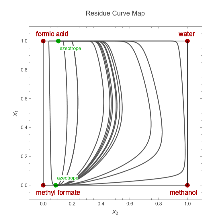
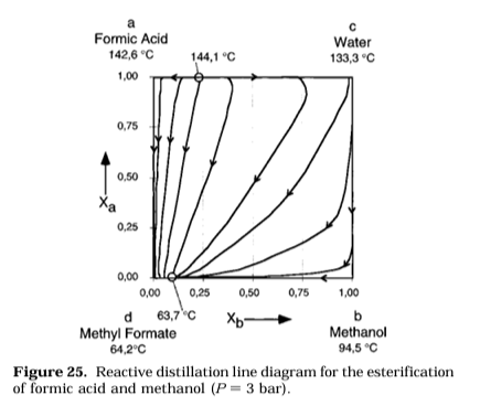
The esterification reaction of methanol and formic acid produces water and methyl formate.The extent of the reaction is limited by the equilibrium constant, taken to be 5.This notebook plots the residue curve passing through several points. It also superimposes the bubble temperature distribution, which indicates that the negative azeotrope between water and formic acid is a stable node with the highest boiling temperature (shown in blue). There is another nonreactive azeotrope in the system between methanol and methyl formate (a positive azeotrope and an unstable node with a low boiling temperature show in magenta). Finally, pure water, methyl formate, methanol, and formic acid are all saddle points. There is only one distillation region in the quaternary diagram.The transformed compositions of the two azeotropes are: A: 0.10478 and 1.0 B: 0.0865 and 0.0The code also displays the iso-temperature curves and the temperature (in °C).References:[1] B. Bessling, G. Schembecker, and K. H. Simmrock, “Design of Processes with Reactive Distillation Line Diagrams,” Industrial and Engineering Chemistry Research, 36(8), 1997 pp. 3032–3042. https://doi.org/10.1021/ie960727p
In[]:=
G1[i_,t_]:=Exp1-Logx[j]A1[i,j,t]-x[j]A1[k,j,t]/.x[3]x3[t]/.x[4]x4[t]/.x[1]x1[t]/.x[2]x2[t];A1[i_,j_,t_]:=V[j]/V[i]Exp[-a[i,j]/(RT[t])];
4
∑
j=1
4
∑
k=1
x[k]A1[k,i,t]
4
∑
j=1
In[]:=
a[1,1]=0.0;a[1,2]=2001.7;a[1,3]=515.9;a[1,4]=-194.6;a[2,1]=80.1;a[2,2]=0.0;a[2,3]=151.7973;a[3,4]=0.0;a[3,1]=74.5;a[3,2]=907.572;a[3,3]=0.0;a[4,3]=0.0;a[4,1]=758.5;a[4,4]=0.0;a[2,4]=0.0;a[4,2]=0.0;
In[]:=
V[3]=40.73;V[4]=37.91;V[2]=61.54;V[1]=18.07;
In[]:=
R=1.987;P=3.0;
In[]:=
Psat1[i_,t_]:=Exp[(Aa1[i]-Ba1[i]/(T[t]-273.15+Ca1[i]))];
In[]:=
Aa1[4]=9.3703;Aa1[2]=10.2965;Ba1[4]=2982.4463;Ba1[2]=2801.0487;Ca1[4]=218.0;Ca1[2]=240.37;Ba1[3]=3643.3136;Aa1[3]=11.9869;Ca1[3]=239.726;Aa1[1]=11.9647;Ca1[1]=233.426;Ba1[1]=3984.9228;
In[]:=
Keq[t_]:=5;
In[]:=
Ksym[t_]:=10^(-18.12+7099/(T[t]));
In[]:=
x2[t_]:=1-x1[t]-x3[t]-x4[t];
In[]:=
sol[p1_,p2_]:=Quiet[FindRoot[{PPsat1[4,t]G1[4,t]x4[t]/((1+Sqrt[(1+4Ksym[t]Psat1[4,t])])/(1+Sqrt[(1+4Ksym[t]Py4[t](2-y4[t]))]))+Psat1[2,t]G1[2,t]x2[t]/((2(1-y4[t]+Sqrt[(1+4Ksym[t]Py4[t](2-y4[t]))]))/((2-y4[t])(1+Sqrt[(1+4Ksym[t]Py4[t](2-y4[t]))])))+Psat1[3,t]G1[3,t]x3[t]/((2(1-y4[t]+Sqrt[(1+4Ksym[t]Py4[t](2-y4[t]))]))/((2-y4[t])(1+Sqrt[(1+4Ksym[t]Py4[t](2-y4[t]))])))+Psat1[1,t]G1[1,t]x1[t]/((2(1-y4[t]+Sqrt[(1+4Ksym[t]Py4[t](2-y4[t]))]))/((2-y4[t])(1+Sqrt[(1+4Ksym[t]Py4[t](2-y4[t]))]))),y4[t]Psat1[4,t]G1[4,t]x4[t]/((1+Sqrt[(1+4Ksym[t]Psat1[4,t])])/(1+Sqrt[(1+4Ksym[t]Py4[t](2-y4[t]))]))1/P,p1x4[t]+x1[t],p2x3[t]+x1[t],G1[1,t]G1[2,t]x1[t]x2[t]-G1[3,t]G1[4,t]x3[t]x4[t]/Keq[t]0},{x1[t],0.01},{x3[t],0.01},{x4[t],0.01},{y4[t],0.2},{T[t],330},AccuracyGoal->20]];
In[]:=
y3[t_]:=Chop[Psat1[3,t]G1[3,t]x3[t]/((2(1-y4[t]+Sqrt[(1+4Ksym[t]Py4[t](2-y4[t]))]))/((2-y4[t])(1+Sqrt[(1+4Ksym[t]Py4[t](2-y4[t]))])))1/P];y1[t_]:=Chop[Psat1[1,t]G1[1,t]x1[t]/((2(1-y4[t]+Sqrt[(1+4Ksym[t]Py4[t](2-y4[t]))]))/((2-y4[t])(1+Sqrt[(1+4Ksym[t]Py4[t](2-y4[t]))])))1/P];
In[]:=
Y1[t_]:=Chop[y4[t]+y1[t]];Y2[t_]:=Chop[y3[t]+y1[t]];
In[]:=
sol1[p1_,p2_]:=First@Quiet[NDSolve[{X1[t]x4[t]+x1[t],X2[t]x3[t]+x1[t],G1[1,t]G1[2,t]x1[t]x2[t]-G1[3,t]G1[4,t]x3[t]x4[t]/Keq[t]0,PPsat1[4,t]G1[4,t]x4[t]/((1+Sqrt[(1+4Ksym[t]Psat1[4,t])])/(1+Sqrt[(1+4Ksym[t]Py4[t](2-y4[t]))]))+Psat1[2,t]G1[2,t]x2[t]/((2(1-y4[t]+Sqrt[(1+4Ksym[t]Py4[t](2-y4[t]))]))/((2-y4[t])(1+Sqrt[(1+4Ksym[t]Py4[t](2-y4[t]))])))+Psat1[3,t]G1[3,t]x3[t]/((2(1-y4[t]+Sqrt[(1+4Ksym[t]Py4[t](2-y4[t]))]))/((2-y4[t])(1+Sqrt[(1+4Ksym[t]Py4[t](2-y4[t]))])))+Psat1[1,t]G1[1,t]x1[t]/((2(1-y4[t]+Sqrt[(1+4Ksym[t]Py4[t](2-y4[t]))]))/((2-y4[t])(1+Sqrt[(1+4Ksym[t]Py4[t](2-y4[t]))]))),y4[t]Psat1[4,t]G1[4,t]x4[t]/((1+Sqrt[(1+4Ksym[t]Psat1[4,t])])/(1+Sqrt[(1+4Ksym[t]Py4[t](2-y4[t]))]))1/P,D[X1[t],{t,1}]-X1[t]+Y1[t],D[X2[t],{t,1}]-X2[t]+Y2[t],X2[0]p1,X1[0]p2,T[0]T[t]/.sol[p1,p2],y4[0]y4[t]/.sol[p1,p2],x1[0]x1[t]/.sol[p1,p2],x3[0]x3[t]/.sol[p1,p2],x4[0]==x4[t]/.sol[p1,p2]},{x1[t],x3[t],x4[t],y4[t],X1[t],X2[t],T[t]},{t,-80,80},AccuracyGoal->5]];
In[]:=
rcm[{p1_,p2_}]:=Quiet@Show[ParametricPlot[Evaluate[{X2[t],X1[t]}/.sol1[p1,p2]],{t,-40,40},PlotStyle{Thickness[0.005],Darker@Gray},PlotRange{{-0.1,1.1},{-0.1,1.1}},FrameLabel{"",""},FrameTrue,AxesOrigin{-0.1,-0.1},ImageSize{450,450},Epilog{Line[{{0,0},{0,1}}],Line[{{0,0},{1,0}}],Line[{{1,0},{1,1}}],Line[{{0,1},{1,1}}]}],Graphics[{Style[Text["methyl formate",{-0.05,-0.05},{-1,0}],Darker@Red,14],Style[Text["formic acid",{-0.05,1.05},{-1,0}],Darker@Red,14],Style[Text["water",{1.03,1.05},{0.6,0}],Darker@Red,14],Style[Text["methanol",{1.03,-0.05},{0.6,0}],Darker@Red,14],Style[Text["azeotrope",{0.115,0.95},{-1,0}],Darker@Green,10,Background->White],Style[Text["azeotrope",{0.096,0.05},{-1,0}],Darker@Green,10,Background->White],Darker@Red,PointSize[0.025],Point[{1,0}],Point[{1,1}],Point[{0,1}],Point[{0,0}],Darker@Green,Point[{0.10478,1}],Point[{0.0865,0}]}]]
X
2
X
1
In[]:=
tbli={{0.72224,0.109449},{0.470703,0.535582},{0.583178,0.293942},{0.165154,0.601258},{0.754218,0.771123},{0.778574,0.0236104},{0.922757,0.992454},{0.350409,0.0450047},{0.501359,0.633756},{0.642208,0.389875},{0.664971,0.843882},{0.238652,0.673513},{0.419507,0.587398},{0.00833523,0.942441},{0.05,0.3}};
In[]:=
RCM=Show[Table[rcm[tbli[[i]]],{i,1,15}],PlotLabel->Style["\nResidue Curve Map\n",14]]
Out[]=