The Casimir effect is a consequence of quantum fluctuations in a vacuum in a bounded region. In this work we solve the Klein-Gordon equation for several boundary conditions and study the dependence of the vacuum energy on the size and shape of the bounded region.
Klein-Gordon Equation in a Cube
Klein-Gordon Equation in a Cube
To obtain a measure of the vacuum energy with respect to external interactions, we are computing the difference between the zero-point energy of space with the applied boundary conditions and the vacuum in its free configuration. It is necessary to apply the Epstein function to regularize the divergent sum of energies of individual modes.
We begin with the Klein Gordon equation
2
∂
∂
2
t
2
∇
2
m
Consider the box:
0<x<, 0<y<, 0<z<
a
1
a
2
a
3
Thus the Dirichlet boundary conditions become:
ϕ(t,0,y,z)ϕ(t,,y,z)0,ϕ(t,x,0,z)ϕ(t,x,,z)0,\[NewLine]ϕ(t,x,y,0)ϕ(t,x,y,)0.
a
1
a
2
a
3
For each,, we have the spatial mode:
For each
n
1
n
2
n
3
u
n
1
n
2
n
3
n
1
a
1
n
2
a
2
n
3
a
3
In[]:=
aValue=1;Plot[Evaluate[Table[Sin[nPiz/aValue],{n,1,4}]],{z,0,aValue},PlotLegends->Table[Row[{"n = ",n}],{n,1,4}],AxesLabel->{"z","u_n(z)"},PlotRange->All,ImageSize->Large]
Out[]=
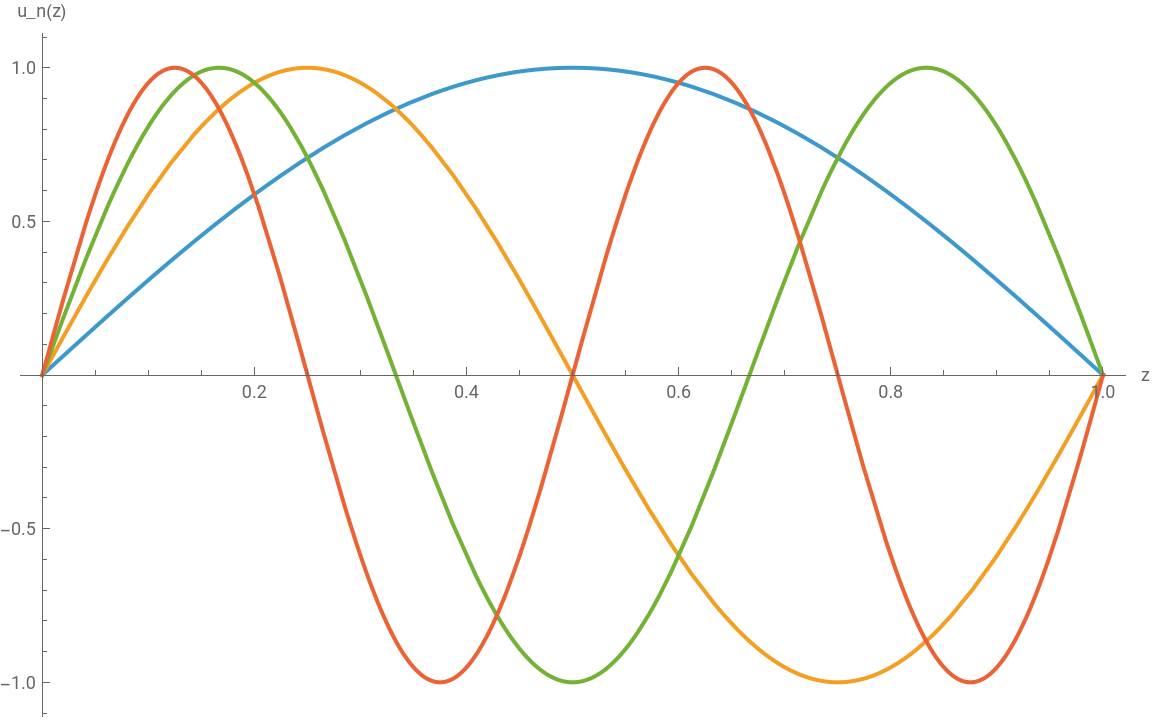


These modes evolve in time as follows:
ϕ
n
1
n
2
n
3
u
n
1
n
2
n
3
-iωt
e
The frequencies of the massless modes read:
ω
n
1
n
2
n
3
2
n
1
2
a
1
2
n
2
2
a
2
2
n
3
2
a
3
These can be obtained by plugging the time-dependent modes in the Klein-Gordon equation and solving for . Let’s check this formula computationally:
ω
In[]:=
u[x_,y_,z_]:=Sin[n1Pix/a1]Sin[n2Piy/a2]Sin[n3Piz/a3];
In[]:=
phi[x_,y_,z_,t_]:=u[x,y,z]Exp[-Iωt];
In[]:=
KG[expr_]:=FullSimplify[D[expr,{t,2}]-D[expr,{x,2}]-D[expr,{y,2}]-D[expr,{z,2}]+m^2expr,Assumptions->Element[{n1,n2,n3},PositiveIntegers]&&Element[ω,Reals]];
In[]:=
kgReduced=FullSimplify[KG[phi[x,y,z,t]]/phi[x,y,z,t],Assumptions->Element[{n1,n2,n3},PositiveIntegers]&&Element[ω,Reals]]
Out[]=
2
m
2
n1
2
a1
2
n2
2
a2
2
n3
2
a3
2
π
2
ω
In[]:=
omegaPositive=Sqrt[kgReduced+ω^2];FullSimplify[kgReduced/.ω->omegaPositive]
Out[]=
0
The total vacuum energy of the massless box is obtained by summing the frequencies of all independent individual modes:
E
0
a
1
a
2
a
3
1
2
∑
n
1
n
2
n
3
ω
n
1
n
2
n
3
π
2
∞
∑
n
1
n
2
n
3
2
n
1
2
a
1
2
n
2
2
a
2
2
n
3
2
a
3
Parallel Infinite Plates
Parallel Infinite Plates
The parallel plate geometry is the simplest setup for studying the Casimir effect. A scalar quantum field is confined between two parallel plates separated by a given distance . As a consequence, the field cannot oscillate freely in the direction perpendicular to the plates, so only certain discrete modes are allowed. Each of the modes contributes to the zero point energy, so restricting the set of allowed modes changes the total vacuum energy.
In 3 dimensions, the frequency satisfies
a
In 3 dimensions, the frequency satisfies
ω
n,
k
T
2
k
T
2
nπ
a
where is the transversal momentum.
k
T
In[]:=
omegaMode[n_,kT_,a_]:=Sqrt[kT^2+(nPi/a)^2];Plot[Evaluate[Table[omegaMode[n,kT,1],{n,1,4}]],{kT,0,10},PlotLegends->Table[Row[{"n = ",n}],{n,1,4}],AxesLabel->{"k_T","omega_n"},PlotRange->All,ImageSize->Large]
Out[]=
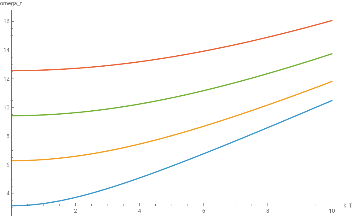
Recall that each allowed field mode contributes to the zero-point energy so we schematically have:
E
0
1
2
As we would expect from the boundary conditions, the momentum normal to the plates is discrete for , and the momentum parallel to the plates is continuous +, so we have a frequency given by +.Thus the energy becomes:
k
z
nπ
a
n1,2,3,…
2
k
T
2
k
x
2
k
y
ω
n,
k
T
2
k
T
2
nπ
a
E
0
1
2
∞
∑
n1
∑
k
x
k
y
2
k
T
2
nπ
a
If the transverse directions were bounded as well, then , . Let area be , then considering the differences we obtain:
k
x
2π
n
x
L
x
k
y
2π
n
y
L
y
A
L
x
L
y
Δ, Δ.
k
x
2π
L
x
k
y
2π
L
y
Taking the infinitesimal limit:
E
0
A
2
∞
∑
n1
2
d
k
T
2
(2π)
2
k
T
2
nπ
a
As this integral is divergent, we introduce a regulator, which we define as:
I(s)-skk-s
1
2
∞
∑
n1
2
d
k
T
2
(2π)
1
2
+
2
k
T
2
nπ
a
1
4π
∞
∑
n1
∞
∫
0
1
2
+
2
k
2
nπ
a
We make the change of variables and so the integral becomes:
u+
2
k
2
nπ
a
du2kk,
∞
∫
0
1
2
+
2
k
2
nπ
a
1
2
∞
∫
2
nπ
a
1
2
u
After computing the integral we obtain:
1
2
∞
∫
2
nπ
a
1
2
u
1
2
∞
-s-s
3
2
u
3
2
2
nπ
a
However, recall that in analytic regularization even though the limit superior diverges we are just left with the lower limit:
1
2
∞
∫
2
nπ
a
1
2
u
1
2
3
2
2
nπ
a
3
2
Thus, the regulator is given by:
By analytic continuation we have:
And we finally arrive at the form:
Thus the energy becomes:
From this we conclude that the vacuum energy between the plates is lower than the energy in the free space.
Hypercube Region
Hypercube Region
where:
Substituting in we obtain:
Solving this expression, the energy is given by:
Similarly to our previous approach, we proceed by analytical continuation the Epstein zeta function is used:
In order to use the Epstein zeta function we need an analogue of the Riemann zeta reflection function in higher dimensions:
In order to use the Epstein zeta function we need an analogue of the Riemann zeta reflection function in higher dimensions:
The energy is given in the form:
The zero point energy then has the form:
Applying the identity
we get
Thus the energy has the form:
Isosceles Triangle
Isosceles Triangle
so the frequencies are
As in the previous cases, we would like to regularize the energy using the analytic continuation of
Concluding Remarks
Concluding Remarks
Acknowledgements
Acknowledgements
I would like to thank my mentors Jesús Montesinos and Pavel Hájek for their technical and technological support throughout this project, my classmates in particular Leyla Kohl for her help in the last moment writing and correcting the English, in the text and colleagues for their valuable comments and suggestions, which greatly enriched this work. My special thanks to Stephen Wolfram for the guidance, encouragement, and support provided during this project. I would like to thank Stephanie Bowyer for her work throughout the program. Being in the WSRI program was an unique experience where I learned a lot and met nice people!
References
References
1
.Ambjørn, J., & Wolfram, S. (1983). Properties of the vacuum: I. Mechanical and thermodynamic. Annals of Physics, 147(1), 1–32.
AI Disclosure
AI Disclosure
During this project, I used ChatGPT to debug some minor functionalities. All code and written content were reviewed, understood, and approved by the author.
CITE THIS NOTEBOOK
CITE THIS NOTEBOOK
Casimir Energy and Geometry
by Pablo Gutierrez
Wolfram Community, STAFF PICKS, July 16, 2026
https://community.wolfram.com/groups/-/m/t/3763708
by Pablo Gutierrez
Wolfram Community, STAFF PICKS, July 16, 2026
https://community.wolfram.com/groups/-/m/t/3763708