ABSTRACT: In classical Kepler problem we assume a perfect point travelling in central Newton (gravity) or Coulomb (EM) potential, leading to well known analytical solutions with elliptic orbits. However, including fixed rotation (of e.g. spinning planet/star, charged object) or magnetic dipole moment (e.g. of particle) for the central or orbiting object, the situation becomes much more complicated as only one angular momentum is conserved. Resulting Lorentz force bends trajectory, allowing to explain why even free-falling objects do not collide, e.g. electrons cannot fall into nucleus. This basic Kepler correction could allow to better understand e.g. Mercury precession, trajectories around rotating stars, or particle scattering scenarios.
DEMONSTRATION: https://demonstrations.wolfram.com/KeplerProblemWithClassicalSpinOrbitInteraction
TALK: https://www.youtube.com/watch?v=zAI_7CbZDsA
DEMONSTRATION: https://demonstrations.wolfram.com/KeplerProblemWithClassicalSpinOrbitInteraction
TALK: https://www.youtube.com/watch?v=zAI_7CbZDsA
This notebook introduces to basic correction of Kepler problem: including rotating/spinning object or dipole. It leads to much more complicated trajectories, one can test in the below demonstration:


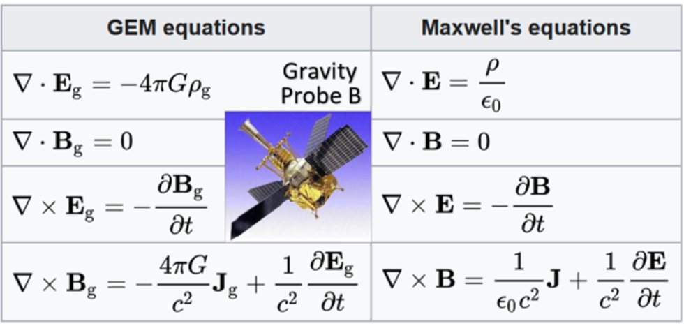
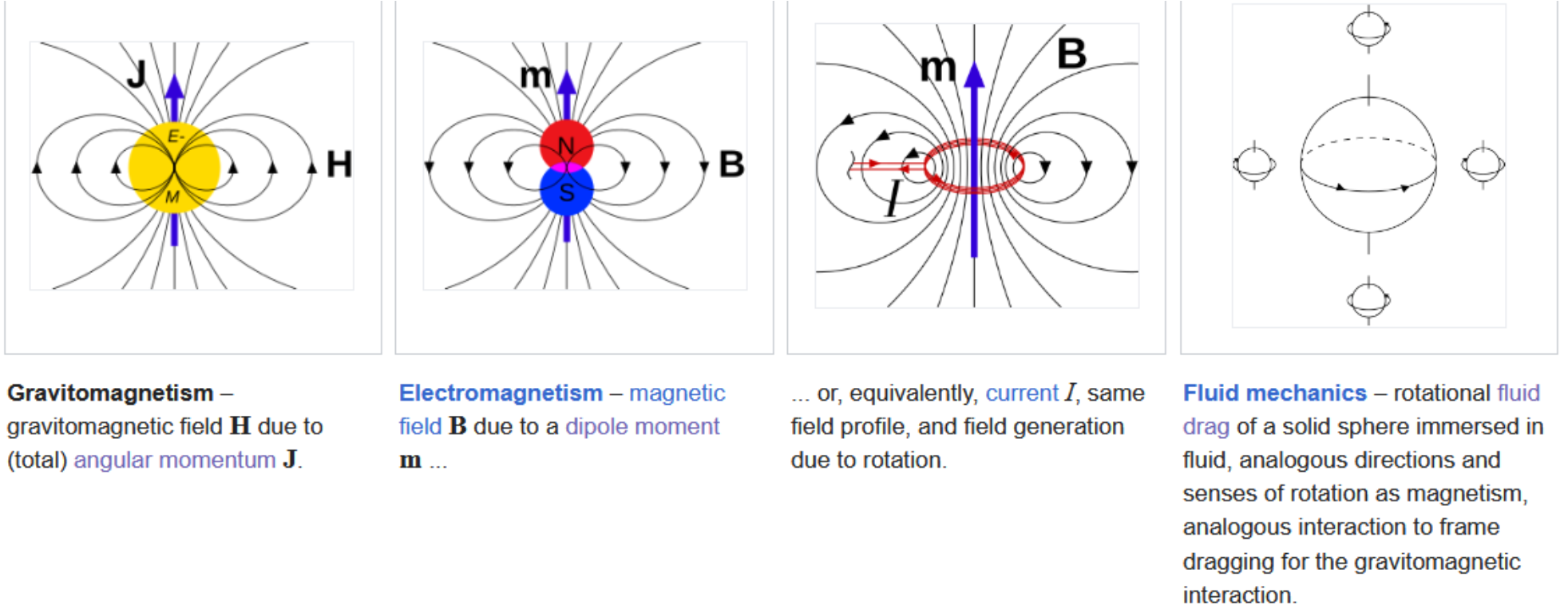
For simplicity we will work in electromagnetic (EM) view: for one of two charged objects having also magnetic dipole moment, like many particles. However, we could alternatively work in gravitoelectromagnetic (GEM) view - second set of Maxwell equations for gravity proposed by Oliver Heaviside in 1893, which was confirmed by Gravity Probe B as approximation of the general relativity, with frame-dragging as analog of the Lorentz force. We need to add magnetism to make Coulomb force Lorentz invariant, the same way GEM extends Newton force for Lorentz invariance by gravitomagnetic field, created e.g. by rotating masses. From GEM view, we discuss Kepler problem for rotating e.g. planet, or around rotating star. Diagrams from https://en.wikipedia.org/wiki/Gravitoelectromagnetism :
Basic Kepler problem in EM view
Basic Kepler problem in EM view
Like in classical Bohr model, still popular e.g. for Rydberg atoms, with electron thousands of times lighter than nucleus, assume we have travelling point-like object of mass , hence (non-relativistic) kinetic energy for ∈ position, ∈, velocity. Assuming it has charge and travels in potential of charge fixed in 0 position, the potential energy is for distance from 0. This way we get Lagrangian: Using Euler-Lagrange: we get standard evolution equation for Z constant and normalized vector position.We can get invariants from Noether’s theorem - here time invariance says energy is conserved: We have also rotation invariance around any axis: for +δ, getting invariance of angular momentum: ()·()·() Here is Mathematica source calculating Euler-Lagrange equations from this Lagrangian and solving numerically, getting elliptic orbits:
m
e
T2
m
e
2
v
r
3
R
v
r
3
R
v
v
-e
Ze
V-Zr
k
e
2
e
r
r
L+
m
e
2
v
2
k
e
Z
2
e
r
d
∂t
∂L
∂
r
∂L
∂r
̈
r
c
e
r
2
r
c
e
k
e
2
e
m
r
r
r
tt+δt
E·v-L-∝-
∂L
∂v
m
e
2
v
2
k
e
Z
2
e
r
2
v
2
c
e
r
n
r
r
n
r
∂L
∂
r
n
r
m
e
v
n
r
m
e
n
r
v
In[]:=
r={x[t],y[t],z[t]};rl=Sqrt[Total[]];v=D[r,t];L=+;(*Lagrangianwithoutconstants:=1*)EL0=Table[D[D[L,v[[i]]],t]==D[L,r[[i]]],{i,3}](*Euler-Lagrangeequations*)
2
r
Total[]
2
v
2
1
rl
c
e
Out[]=
[t]-,[t]-,[t]-
′′
x
x[t]
3/2
(++)
2
x[t]
2
y[t]
2
z[t]
′′
y
y[t]
3/2
(++)
2
x[t]
2
y[t]
2
z[t]
′′
z
z[t]
3/2
(++)
2
x[t]
2
y[t]
2
z[t]
{sol=NDSolve[Join[EL0,{x[0]==1,y[0]==0,z[0]==0,x'[0]==0,y'[0]==1,z'[0]==0}],{x,y,z},{t,0,10}][[1]];ParametricPlot3D[r/.sol,{t,0,10}]}
Out[]=

Adding magnetic dipole moment
Adding magnetic dipole moment
Now assume one of the two charged objects have also magnetic dipole moment, e.g. μ for particle with spin, can be also from rotation of charged objects, or massive in GEM. It leads to () and magnetic field as below, with drawn vector fields:
m
s
A
r
μ
0
4π
m
r
2
r

In[]:=
s={0,0,1};r={x,y,z};rl=Sqrt[Total[]];rh=r/rl;VectorPlot3D[Cross[s,rh],{x,-1,1},{y,-1,1},{z,-1,1},PlotLabel->"A field"],VectorPlot3D[(3rh(s.rh)-s),{x,-1,1},{y,-1,1},{z,-1,1},PlotLabel->"B field"]
2
r
2
rl
3
rl
Out[]=
 ,

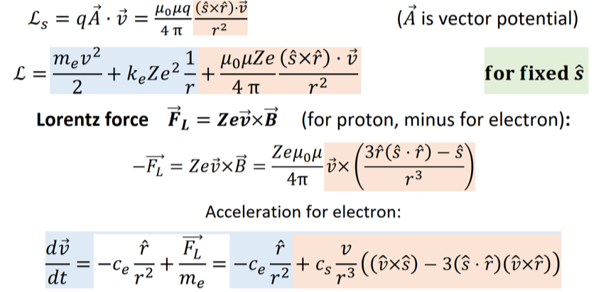
Lagrangian contribution for velocity charge in field is q·. While generally direction of spin can vary, for simplicity assume here it is constant (0,0,1), leading to below Lagrangian, Lorentz force, acceleration:
v
q
A
L
s
A
v
s
s
Numerical simulations
Numerical simulations
General trajectories
General trajectories
CITE THIS NOTEBOOK
CITE THIS NOTEBOOK
Kepler problem with spinning object or dipole
by Jarek Duda
Wolfram Community, STAFF PICKS, August 1, 2025
https://community.wolfram.com/groups/-/m/t/3522853
by Jarek Duda
Wolfram Community, STAFF PICKS, August 1, 2025
https://community.wolfram.com/groups/-/m/t/3522853