This essay was written by Margaux Wong as part of the Wolfram Emerging Leaders Program for Undergraduates, which is a 5-month long, project-based program designed for undergraduate students to take a deep dive into a topic of their choice. Students work remotely to take their project from ideation to completion, with the guidance of Wolfram experts.
Abstract
Abstract
Multiway Sequential Cellular Automata (MSCA) are an asynchronous, multi-branching version of classical cellular automata. This study investigates the underlying behavior of these MSCA through an examination of the impact of array length and branching possibilities. MSCA of array length nine were compared with previous work on arrays of length six to expand class definitions. Direct graph comparison enabled more advanced definitions of class graph structure, while rule frequency analysis and a novel approach, normalized target distribution ratio (NTDR) analysis, clarified class similarities and highlighted five underlying graph subclasses of Class 10 Lattices. Rule frequency analysis revealed rule patterns that differentiated between classes. NTDR analysis revealed four groups of classes and subclasses based on target distribution. The NTDR highlighted ruleset characteristics that caused respective graph structures. This study also extended previous work on two-branch MSCA to broader branching cases, namely the Quad Flex which allows for varying numbers of branches between one to four per node, and presents initial findings on resulting deterministic graph features.
Introduction
Introduction
Cellular Automata (CA) are discrete models of computation. In the one-dimensional, binary case, CA consist of an array of binary cells defined by an initial state and a list of evolutionary rules. Multiway Sequential Cellular Automata (MSCA) are an asynchronous, multi-branching version of classical cellular automata [1, 2]. Local updating of cell values in a sequential manner uses updated values in each step, and every updating step can have multiple end values necessitating the use of graph structures to display the evolution of array values. The following table shows the progression of an MSCA through multiple steps and generations, or a complete set of update steps over the entire array. Each column is a full generation of evolution, meaning all cells in the array have been updated. Each element of the table is a single asynchronous step of a full generation.
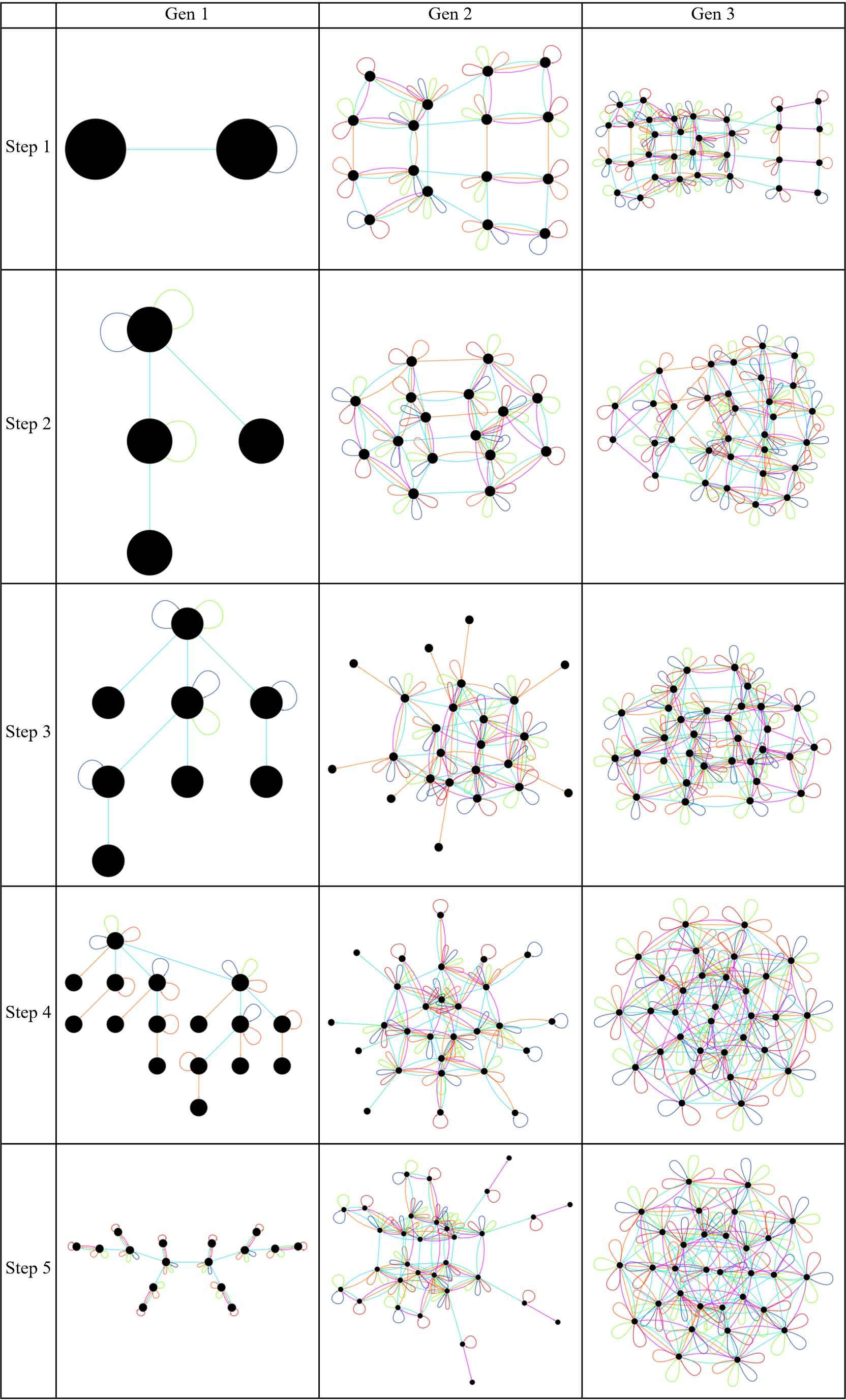
This work focuses on the two-cell version of the MSCA where the rule set takes two adjacent cells as inputs and yields multiple pairs of cells as outputs. The updating scheme of the MSCA within generation . Let be a finite array of length N that denotes the state of the array after application of the rules in step of generation in branch . Let be the input cell values, be the target cell values, and h the function that defines the rule sets being applied by this particular MSCA. The mapping then can be expressed as follows where is the maximum number of branches allowed at each step, indicates the current element of the set of inputs, is the th element of (i.e. one of the inputs), indicates the number of branches or mappings that occur for element , and is the cardinality of . Let be the branch of the tree from the previous generation, whose descendants are being constructed.
gcanbedescribedasfollows
a
j,s,g
s
g
j,thecurrentbranchbeingconstructed
I
T
h
b
k
I
k
k
I
J
k
I
k
D
I
h:{}fork∈,1≤k≤Dand∈{1,...,b}
I
k
J
k
T
J
k
q
When for 1 ≤ ≤ , where is determined by the value of input cells,
s>1,
j
J
k
k
[s],[s+1]=h[s],[s+1]fori=sandi=s+1[i]=[i]fori!=sandi!=s+1
a
j,s,g
a
j,s,g
a
q,s-1,g
a
q,s-1,g
a
j,s,g
a
q,s-1,g
When s = 1, for 1 ≤ ≤ , where is determined by the value of input cells, the updated values are based on the last step of the previous generation, .
j
J
k
k
s=N-1
g-1
[s],[s+1]=h[s],[s+1]fori=sandi=s+1[i]=[i]fori!=sandi!=s+1
a
j,s,g
a
j,s,g
a
q,N-1,g-1
a
q,N-1,g-1
a
j,s,g
a
q,N-1,g-1
The M-type rule sets used by the MSCA for a two cell input, two cell output structure have four possible outputs for each input as shown in the following table. Thus, there are 16 possible basic rules. Each of these rules has been color coded as shown in the first example to allow the impact of these individual rules to be seen in state graphs. An M-type rule set is a subset of these 16 rules.

This work examines the effect of various parameters on the MSCA including array length and expanding the multiway system to include up to four branches.
Array Length
Array Length
In previous work, an array of length six was used as the input array to the MSCA [2]. This work examines the effects of increasing this length to nine while remaining a two-branch multiway system at each node. Longer arrays were experimented with, however, the state graphs quickly grew too large to be rendered. By examining the effect of the MSCA on longer arrays, characteristics of the classes of graphs can be seen in more detail.
As shown in the previous table, there are four possible outputs for each input, namely, 00, 01, 10, and 11. A rule set for a two-branch MSCA contains two of these four possible outputs for each input, for example, 00 could target 01 and 10 or 00 and 10, but not 00, 01, and 10. The two target pairs of cells are required to be distinct. Thus, the first output has four choices and the second output has three choices. This yields 12 possible pairs of distinct outputs. However, within these 12 possible pairs, each pair has a duplicate, in other words, the set of 12 pairs contains both xy mapping to ab and cd, as well as xy mapping to cd and ab for each combination. Removing these duplicates gives six possible output cell pairs for each input cell pair. Since there are four input cell pairs, this results in or 1296 possible rule sets. These 1296 rule combinations will be referred to as M-type rule sets, where a number specifies the identity of each particular rule set, to distinguish them from both the 16 possible input-output cell level rules shown in Table 2, as well as the standard CA rules [2, 3].
As shown in the previous table, there are four possible outputs for each input, namely, 00, 01, 10, and 11. A rule set for a two-branch MSCA contains two of these four possible outputs for each input, for example, 00 could target 01 and 10 or 00 and 10, but not 00, 01, and 10. The two target pairs of cells are required to be distinct. Thus, the first output has four choices and the second output has three choices. This yields 12 possible pairs of distinct outputs. However, within these 12 possible pairs, each pair has a duplicate, in other words, the set of 12 pairs contains both xy mapping to ab and cd, as well as xy mapping to cd and ab for each combination. Removing these duplicates gives six possible output cell pairs for each input cell pair. Since there are four input cell pairs, this results in
4
6
Classes
Classes
In the original work, state graphs were classified into 10 classes based on structure [2]. This paper examines the MSCA with an initial condition of 000111000. In examining this N=9 case, some of these classes become more distinct while others show divergence into several subclasses.
Radials
Radials
The following figure shows the exemplar of the Class 1 Radial graphs from the N=6 dataset. The subsequent figures in this subsection show graphs with N=9 that were also classified as radials.
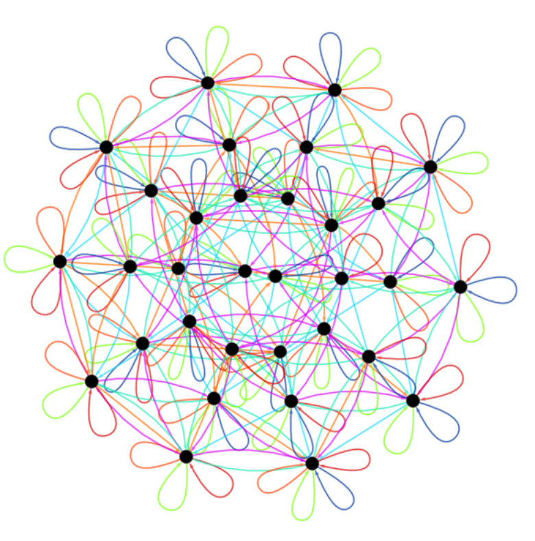
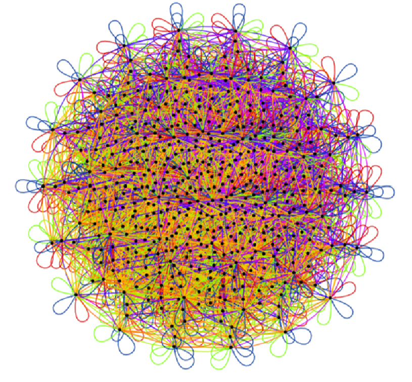
Comparing the exemplar from the N=6 dataset to the first N=9 radial graph shown above, a similar radial structure is seen. This particular graph has two primary colors representing two rules from the table in the introductory section. The overall structure remains very similar, though the density is naturally much greater due to more states and more steps before convergence.
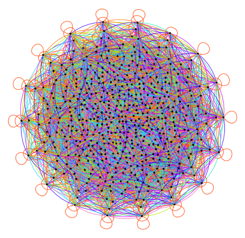
The N=9 graph above is more uniform in terms of color than the previous graph and more closely resembles the N=6 exemplar. It retains the overall structure of the exemplar, but its radial structure is harder to detect due to the number of edges in the graph.
Lattices
Lattices
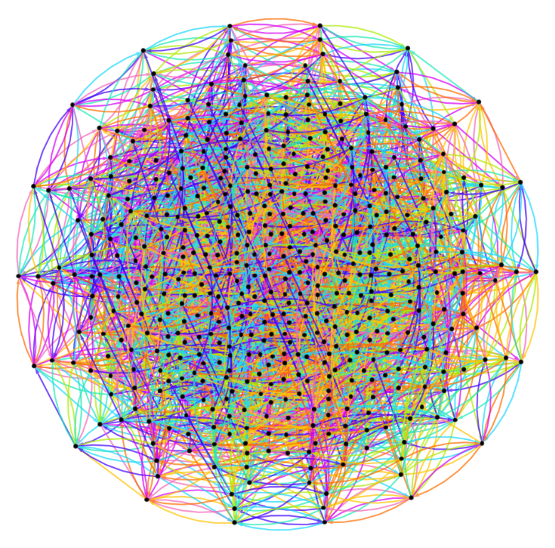
The most interesting class to examine are the Class 10 Lattices. In previous work, it was hypothesized that there existed subclasses of Lattices because the rule frequency analysis showed more uniformity across rules, meaning all rules were applied at a similar rate. This was an outlier compared to other classes and hinted at subclasses with different underlying structures. In the N=9 case, this became apparent as lattice structures became more fully developed. The following figure shows the exemplar for the class from the N=6 original dataset. The next five figures show examples of the distinct subclasses that have emerged through this N=9 study.
The above figure most closely resembles a more developed version of the exemplar, both in structure and color scheme. The central structure is clear and there are large sparse regions on both sides. The fewer number of edges and chain-like structure shows that the behavior of the MSCA under this ruleset was less complex compared to other classes with a dense structure of edges and nodes. The overall structure is reminiscent of a butterfly.
This figure, while still having the sharp protrusions, has a far larger mass of nodes and edges in the center of the graph. Additionally, the protruding edges are shorter compared to the large arcs in the previous figure. The center mass of nodes and edges is so dense it is difficult to observe structures within. This does have some similarity to the center mass structure of the previous figure in overall structure but is distinct enough to warrant a subclass.
This figure is quite different from the other Lattice graphs. It has a concentrated small pink and purple section attached to a larger blue section with sparser edges. Interestingly, this structure bears some resemblance to the Fish Class found in Multiway Circular Sequential Cellular Automata [1]. If the blue edges were also found on the opposite side of the center mass, this figure would more closely resemble both the exemplar and the first N=9 lattice graph however it’s skewed character again warrants a subclass.
The structure in this figure appears to be a graph structure from Class 6 Periodic structures with added large spikes containing an edge to an outlier node and another two edges connecting back to the central mass. Upon very close inspection, the first two N=9 figures appear to possibly contain four groupings in the center structure, aligning with this figure. However, the pronounced nature of the four groupings yields another subclass.
Similarly, the structure in this figure resembles a Class 5 Bimodal graph with additional spikes. The two main masses can be clearly observed. As this structure is unique in its bimodal nature, it again forms a subclass of Lattice graphs.
Rule Frequency Analysis
Rule Frequency Analysis
Rule frequency analysis can provide insight into underlying behavior in state graphs. Within a class, the frequency of each of the 16 basic rules described in the table in the introduction can be determined as follows. Each graph in the class is created with a particular M-type rule set. This rule set consists of 8 basic rules. A tally is made of all of the basic rules used in each graph in each class. The number of occurrences of a particular basic rule across all the rule sets that generate the graphs in the class is then normalized by the total number of basic rules across all the graphs in the class to yield the rule frequency. The functions necessary to calculate and display this analysis are below. In the following bar charts, the 16 basic rules are displayed on the x-axis, and the frequency of each is shown on the y-axis. The colors of the bars correspond with the colors of each rule application in the state graphs.
Normalized Target Distribution Ratio Analysis
Normalized Target Distribution Ratio Analysis
The NBTD describes the likelihood of any given M-type rule set having a certain TD. The number of graphs corresponding to each TD for every class was determined, then, these counts were normalized by the size of the class to find the normalized class target distribution value (NCTD). Since this analysis focused on target distributions, the size of classes was insignificant.
Each NCTD was normalized by the NBTD to achieve the normalized target distribution ratio (NTDR).
An NTDR value of one for a particular TD indicates that the number of graphs in the specified class with that TD aligns with the expected number given the NBTD. A larger NTDR demonstrates a higher number of graphs than expected, while a lower value means fewer graphs resulted from the TD than expected. Ultimately, analyzing the NTDR as a function of graph class enables analysis of the relationship between particular TDs and classes, along with highlighting similarities and differences between classes. The functions needed to calculate and display the NTDR are below. The following bar charts display the results of the NTDR analysis for each class and, if applicable, class subclasses. The x-axis shows the eight base TD cases and the y-axis is the NTDR for that particular TD.
There are several instances in which two target analyses presenting the same indicates the similarity between classes. For example, the first Axial subclass is very similar to the Even target analysis. For both classes, the 4211 and 3311 target distributions are prevalent, and the 3221 and 2222 target distributions are somewhat prevalent. The Skewed and Central target analyses are also similar, having a larger NTDR for the 2222, 3221, 3311, and 4211 target distributions. Although the relative scales of the four aforementioned target distributions varies, the Grid target analysis can also be considered in the broader group of the Axial 1, Even, Skewed, Cluster, Grid classes with a strong prevalence of the 4211 target distribution.
The extremely structured Bimodal, Radial, and Periodic classes all demonstrate a large NTDR for the 2222, 3221, and 3311 target distributions. These three classes show a distinct lack of the 4211 target distribution, distinguishing them from the Axial 1, Even, Skewed, Cluster, Grid group. Further investigation into the structural impact of the 4211 target distribution is necessary. The 2222, 3221, and 3311 target distributions are the most balanced with respect to the possible targets, and are far more balanced than the target distributions discussed regarding Lattices below. These three target distributions limit the MSCA the least during evolution, and drive final graph structures that include densely packed edges and nodes with fewer highly deterministic parts of the graph.
Two distinct groups form within the five Lattice subclasses. The first and fifth Lattice subclasses are extremely similar, with an unusually high usage of the 4400 target distribution. Compared to the other classes where maximum NTDRs range from 1.5 to 5, an NTDR of ~12 and 14 for the first and fifth subclasses, respectively, is outsized. This distribution is unique because there are exactly two targets in the rule set. In other words, all evolutionary steps must transform the current pair of cells into one of two possible cell pairs. This limits the behavior of the MSCA, creating fewer edges during evolution, encouraging deterministic behavior, and decreasing the number of steps to convergence. The structure of these graphs reflects this behavior, namely, the long deterministic chains and few number of edges persistent in the graphs.
The second, third, and fourth Lattice subclasses are similar, and form a second subgroup of Lattices. All three subclasses have a prominent target distribution of 3320, and somewhat prominent target distributions of 4220 and 4310. The NTDR analysis shows that there are a handful of 4400 outliers in the second Lattice subclass that belong in either the first or fifth Lattice subclass instead. However, disregarding these outliers, leaves the target distributions 3320, 4220, and 4310, which are the three target distributions with only three total targets. This limits the behavior of the MSCA, but not as much as the first Lattice subgroup. The Lattice class overall thus consists of MSCA where the rule set does not contain all four target possibilities (00, 01, 10, 11).
The second Axial subclass does not have clear results from this target analysis, which indicates that this subclass requires an additional layer of subclasses. Across classes, there are several instances of extremely low NTDRs that are nonzero. These show the margin of error resulting from classification of the graphs. The overall analysis of the relative ratios of NTDRs for each class is much broader than this margin of error, thus it remains a valuable tool of analysis.
Ultimately, there are four groups of classes and subclasses that result from this NTDR analysis.
1
.The group shown by the first and fifth Lattice subclasses, distinguished by its prevalence of rule sets with only two targets.
2
.The group shown by the second, third, and fourth Lattice subclasses, distinguished by its prevalence of rule sets with only three targets.
3
.The group shown by the Radial, Periodic, and Bimodal classes, distinguished by its prevalence of rule sets with balanced targets.
4
.The group shown by the first Axial subclass and the Central, Grid, Skewed, and Even classes, distinguished by its prevalence of rule sets with balanced targets and the 4211 target distribution.
Expanding Dimensionality: Quad Flex Case
Expanding Dimensionality: Quad Flex Case
Let b denote the dimensionality of MSCA rule sets. The subsection of MSCA examined previously were MSCA where b = 2. This work extends to the b ≤ 4 case that allows for one, two, three, and four possible outputs per input cell pair, and is called the Quad Flex. This scenario contains a total of 50625 rule sets. Selected examples of Quad Flex graphs are shown below.
Determinism in Quad Flex State Graphs
Determinism in Quad Flex State Graphs
The following figures are examples of Quad Flex graphs that do not fit into any of the existing ten defined classes. Long chains of nodes with only one edge between them are deterministic, and result from rule sets with only one possible output cell pair for an input cell pair. Deterministic behavior is correlated with earlier convergence because there are fewer behaviors possible.
Quad Flex Graphs in Existing Classes
Quad Flex Graphs in Existing Classes
Despite the increased number of branches at each node and the flexibility of nodes having one, two, three, or four branches as opposed to a specified number of branches, a significant portion of the Quad Flex graphs fall into existing defined classes. The following figures show graphs from the set of 50625 Quad Flex graphs that belong in the existing Radial, Central, Skewed, Bimodal, Periodic, Grid, and Even classes, respectively.
Conclusion and Future Work
Conclusion and Future Work
This study examined the effects of varying array length and branching possibilities on MSCA behavior and class features through a variety of methods. State graphs were generated for all 1296 rule sets using an array of length nine, then classified. Class definitions were expanded through a comparison with previous work on arrays of length six MSCA. Rule frequency analysis was performed on all the classes and two distinct sets of influential basic rules emerged that indicated relationships between classes and subclasses. A novel approach, normalized target distribution ratio (NTDR) analysis, which examines the behavior of rule sets as a whole, was then performed on the classified data. Two overall groups of Class 10 Lattices emerged from the five Lattice subclasses, and two additional groups based on prevalence of the 4211 target distribution resulted from the other classes with more balanced target distributions. NTDR analysis also highlighted the target mechanism behind differentiating graph behaviors. A separate Quad Flex group of 50625 MSCA resulting from broadening the two-dimensional constraint of existing MSCA were simulated then examined, revealing new deterministic graph features.
Further work on the 4211 target distribution as well as correlation of NTDR analysis with convergence rates is necessary, along with further analysis of the Quad Flex graphs resulting from the expansion of dimensionality.
Further work on the 4211 target distribution as well as correlation of NTDR analysis with convergence rates is necessary, along with further analysis of the Quad Flex graphs resulting from the expansion of dimensionality.
Acknowledgements
Acknowledgements
I would like to thank Stephen Wolfram for the inspiration to work on this topic. I would also like to thank Hatem Elshatlawy and Lyman Hurd for invaluable mentorship and Rory Foulger for unbridled support.
References
References
1
.Wong, M. (2022, July). Multiway sequential cellular automata. https://community.wolfram.com/groups/-/m/t/2580859
2
.Wong, M. (2023, Feb). Characterization of Multiway Sequential Cellular Automata. https://community.wolfram.com/groups/-/m/t/2838403
3
.Wolfram, S. (2002). A New Kind of Science. Wolfram Media.
CITE THIS NOTEBOOK
CITE THIS NOTEBOOK
Analysis of multiway sequential cellular automata: Class evolution and quad flex case
by Margaux Wong
Wolfram Community, STAFF PICKS, January 30, 2025
https://community.wolfram.com/groups/-/m/t/3367501
by Margaux Wong
Wolfram Community, STAFF PICKS, January 30, 2025
https://community.wolfram.com/groups/-/m/t/3367501