Speedup and Slowdown Phenomena in Turing Machines

function

1

states

2

3

4

(2,2) #TMs = 4; #Algs = 2

σ

i

τ

i

<σ>

<τ>

<σ+2

>

h

<τ

>

h

This Demonstration shows how on average using more states in a Turing machine (TM) leads to slower-running algorithms to compute the same function. Use the slider "function" to choose between the 21 functions that occur in the three explored Turing machine spaces with two symbols and two, three, and four states.

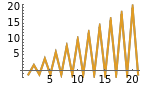
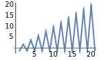
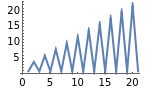
The diagrams show how much tape space and how much time the Turing machines used to compute each function with different states. The first column of diagrams with

σ

refers to how many tape cells were used by the TM. The second column displays how many computation steps were needed before the TMs finished their computation. For example, the

τ

i

plots the time usages for each Turing machine; the

<τ>

diagram plots the average time usage, and the

<τ

>

h

diagram shows the harmonic average (as a measure of average information) computed in a unit of time. Function 8, for example, is the function that just deletes the first black input cell; you can see that there are Turing machines with three and four states that compute function 8 in exponential time.

On the left, a visual representation of the computed function is given. You should read it as a sequence of rows, where each row represents an output tape configuration. The top row is the output (as a tape configuration) of the TM when it started with just one black cell. The next row below it is the tape configuration that is output by the TM after feeding it two consecutive black cells etc. Our TMs compute with only black and white cells and do not use other colors. A red tape indicates that the TM did not halt on the corresponding input. You can choose the number of states to be 2, 3, or 4.