CITE THIS NOTEBOOK: An open problem: explaining inconsistency in hard spheres dynamics by Hanfeng Zhai. Wolfram Community MAR 14 2023.
I’m writing this short essay to post an open question and hope to seek intelligence from the community trying to explain an abnormal phenomenon I observed initially during my winter school project. I hope this effort may lead to some contributions toward the understanding of hard sphere modeling of particle systems in the field of statistical physics. I observe that as one changes the particle radii simultaneously pertaining to the same volume fraction, there is an inconsistency in the collision rate-temperature slope as the largest and smallest particle radii (by our definition) seem to have the same slope whereas the middle regime possesses a different slope. Such a phenomenon is highly unexpected and bothers me in the past few weeks/month. I proposed an explanation (or just a rough guess) based on my physics intuition stating that when the radii of the particles are in the middle (between the smallest and largest under the coarse-grain assumption), the particle systems undergo the sub-diffusion process, leading to the inconsistency. I hope to get feedback from experts in the communities.
Definition & Formulation
Definition & Formulation
Following my winter school project, there is one specific problem that really bothers me in my hard sphere simulations for a long time and I have not yet come up with any rigorous and examinable explanations, although I do have some guesses. At this stage, I believe I don’t really have too much brightness to rigorously explain this so I decided to write a short computational essay to explain this problem and hope to elicit future works in the field.
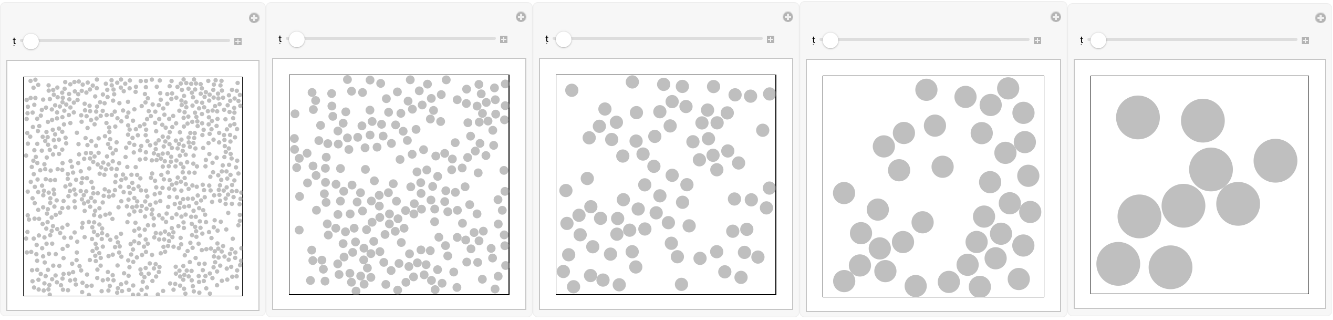
I first come up with a definition of coarse-graining (details please check my winter project), performing resize of the particles in a constrained box simultaneously pertaining to the same volume fraction. Under this definition of the so-called coarse-graining process, we are reducing the system’s order so that one can perform simulations much faster by assuming a larger particle represents many smaller particles. Following this definition and our original formulation of CG, we define the following five systems representing five different degrees of coarse-graining.
Assume5differentdegreesofcoarsegraining.Assumingafinesystemwithparticles.DenotetheoriginalsystemassystemA,thissystemcanalsobecoarse-grainedinto(B):particles;(C):particles;(D):particles;(E):particles.AssumingsystemEhasaboxsizeof10,thecorrespondingboxsizesforthefourothersare(A);(B);(C);(D).Wecanthentestthephysicsofthefoursystemsandcheckwhethertheyagreewiththeidealgaslawwiththesamefittingcoefficients.
3030900
105
1515225
103
9981
102
6636
101
339
101000
900
9
10250
225
9
1090
81
9
1040
36
9
In[]:=
vizsysA=ResourceFunction["HardSphereSimulation"][<|"Positions"->"RandomNonOverlapping","Velocities"->RandomPoint[Ball[{0,0},1],900],"BoxSize"->10,"StepSize"->0.5,"ParticleRadius"->0.1,"Steps"->1,"BoundaryCondition"->"Reflecting","Output"->"Visualize"|>];vizsysB=ResourceFunction["HardSphereSimulation"][<|"Positions"->"RandomNonOverlapping","Velocities"->RandomPoint[Ball[{0,0},1],225],"BoxSize"->10,"StepSize"->0.5,"ParticleRadius"->0.2,"Steps"->1,"BoundaryCondition"->"Reflecting","Output"->"Visualize"|>];vizsysC=ResourceFunction["HardSphereSimulation"][<|"Positions"->"RandomNonOverlapping","Velocities"->RandomPoint[Ball[{0,0},1],81],"BoxSize"->10,"StepSize"->0.5,"ParticleRadius"->0.3,"Steps"->1,"BoundaryCondition"->"Reflecting","Output"->"Visualize"|>];vizsysD=ResourceFunction["HardSphereSimulation"][<|"Positions"->"RandomNonOverlapping","Velocities"->RandomPoint[Ball[{0,0},1],36],"BoxSize"->10,"StepSize"->0.5,"ParticleRadius"->0.5,"Steps"->1,"BoundaryCondition"->"Reflecting","Output"->"Visualize"|>];vizsysE=ResourceFunction["HardSphereSimulation"][<|"Positions"->"RandomNonOverlapping","Velocities"->RandomPoint[Ball[{0,0},1],9],"BoxSize"->10,"StepSize"->0.5,"ParticleRadius"->1,"Steps"->1,"BoundaryCondition"->"Reflecting","Output"->"Visualize"|>];
In[]:=
Row[{vizsysA,vizsysB,vizsysC,vizsysD,vizsysE}]
Out[]=
Approach & The Problem
Approach & The Problem
Now we want to prove (at least we expect) that the collision-temperature diagrams are the same since we consider all these systems are surrogates of each other. Following up on our original formulation, the boundary conditions (BCs) also matter in defining coarse-graining. If we set the BCs as reflective, then the assumption can be considered as “strictly coarse-grain”: each larger particle of a larger radius represents many smaller particles. However, if we set the BCs as periodic, the definition can be more flexible: the large particles’ system can be considered as the “zoomed-in” view of the smaller particle system, or a general sense of representative volume unit (RVE). It can also be interpreted as a coarse-grained system, similar to that of the reflective BCs.
With these more flexible simulation settings, we hope to revisit our simulations back in the winter school project and see whether there are any changes in the results of the collision processes.
We can first define a function to output the collision and temperature from the defined particle simulations, the only difference here would be the BCs as we previously discussed:
In[]:=
TempVsCRcoarsegrain[v_,bs_,num_]:=Module[{dataset,temp,finals,finaltime,cr},(*Compute dataset*)dataset=ResourceFunction["HardSphereSimulation"][<|"Positions"->"RandomNonOverlapping","Velocities"->RandomPoint[Sphere[{0,0},v],num],"BoxSize"->bs,"StepSize"->0.1,"ParticleRadius"->1,"Steps"->5000,"ParticleMass"->(1/bs)*ConstantArray[1,num],"BoundaryCondition"->"Periodic","Output"->{"Collisions","Temperature"}|>];(*Compute temperature*)temp=First[dataset[[2]]];(*Extract collision rate (next three lines)*)finals=MaximalBy[dataset[[1]],#[[3]]&];finaltime=First[finals][[3]];cr=Length[dataset[[1]]]/finaltime;(*Return both temperature and collision rate*){temp,cr}]
Then we run the same simulation as before and test the collision rate-temperature relationship.
In[]:=
paramsweepA=ParallelMap[TempVsCRcoarsegrain[#,900,900]&,Range[0.1,1,0.05]];paramsweepB=ParallelMap[TempVsCRcoarsegrain[#,225,225]&,Range[0.1,1,0.05]];paramsweepC=ParallelMap[TempVsCRcoarsegrain[#,81,81]&,Range[0.1,1,0.05]];paramsweepD=ParallelMap[TempVsCRcoarsegrain[#,36,36]&,Range[0.1,1,0.05]];paramsweepE=ParallelMap[TempVsCRcoarsegrain[#,9,9]&,Range[0.1,1,0.05]];
After the computation (which takes a very long time), we can then plot the relationship between the collision rate to the square root of the temperature, shown in the following diagram. We hope to check whether the fits agree with each other as the physical systems can be considered as “coarse-grained”.
In[]:=
ShowListPlot(1/30)
#[[1]]
,(1/900)#[[2]]&/@paramsweepA,PlotStyle->Red,PlotRange->{{0,0.1},{0,0.5}},ListPlot(1/15)#[[1]]
,(1/225)#[[2]]&/@paramsweepB,PlotStyle->Blue,PlotRange->All,ListPlot(1/9)#[[1]]
,(1/81)#[[2]]&/@paramsweepC,PlotStyle->Green,PlotRange->All,ListPlot(1/6)#[[1]]
,(1/36)#[[2]]&/@paramsweepD,PlotStyle->Orange,PlotRange->All,ListPlot(1/3)#[[1]]
,(1/9)#[[2]]&/@paramsweepE,PlotStyle->Brown,PlotRange->AllOut[]=
Similar phenomena have been observed: the relationships are not consistent for different coarse-grained systems. The slope for the brown dots (system E) is evidently larger than the others. It can be roughly observed that the orange, green, and blue dots seem to preserve the same slope (systems B, C, and D). To verify this observation, we then visualize the relationship between collision rate vs. temperature in the double logarithmic plot, shown as follows:
In[]:=
ListLogLogPlot[{(1/900)paramsweepA,(1/225)paramsweepB,(1/81)paramsweepC,(1/36)paramsweepD,(1/9)paramsweepE},PlotLegends->{"System A","System B","System C","System D","System E"},FrameLabel->{Style["Temperature",Black,16],Style["Collision Rate",Black,16]},PlotStyle->{Red,Blue,Green,Orange,Brown},Frame->True]
Out[]=
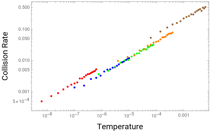


From both the two figures it can be obviously detected that system. A & E, and system. B, C & D seem to behave the same - yet A, B, C, D, E, seem not to coincide with each other. This abnormal phenomenon bothers me for a while and I’m simply not bright enough to come up with a thorough and rigorous explanation. One can then try to change certain parameters in the previous sweep and function implementation part, but after tuning the parameters in the simulations the same behavior still occurs. After digging into the physics of this phenomenon, I have some naïve thoughts that may explain part of the phenomenon. However, my best hope is researchers reading this report could come up with more insightful comments or explanations.
What are My Guesses?
What are My Guesses?
Relationships between CR vs. Temperature to MSD vs. Time
Relationships between CR vs. Temperature to MSD vs. Time
Literature Results & Discussions
Literature Results & Discussions