Understanding how the brain functions and its associated neurological disorders has a crucial impact on human health. Existing computational methods modeling brain functions are accurate, but are often computationally inefficient and cannot be implemented at the complexity of a human brain. To improve the efficiency of brain modeling, I used cellular automata to model neural firing patterns. I modeled both normal and abnormal brain activity using cellular automata. When measuring the number of neurons firing as a measurement of brain activity, the neurons displayed behavior similar to those measured by electroencephalograms. Additionally, when modifying parameters to reflect abnormal brain conditions, the model also displayed abnormal behavior associated with neurological conditions such as epilepsy. Overall, I found that a simple neural model using cellular automata is capable of simulating behavior associated with both normal brain function and neurological conditions. While this project was conducted on a small scale, it shows that neuron models can be simplified computationally while still resembling realistic brain behavior.
Introduction
Introduction
Computational modeling of the brain is an important area of neuroscience research in order to better understand human brain function and the pathology of neurological diseases such as epilepsy, Alzheimer’s, and Parkinson’s. By varying the parameters of the model, researchers can study the impact of certain factors on brain activity. Current computational models of neurons are accurate, but not computationally efficient. For example, the neural model run at the Fugaku supercomputer has accurately modeled a network of 9 million neurons; however, improvements can be made to increase the computational efficiency and the scale of the model, as the model still took significant time to simulate just one second of brain behavior (Kuriyama et al., 2025). Computationally efficient ways of modeling neurons will provide insights on a macroscopic level and will show how complex behaviors arise from individual neurons. Cellular automata is an efficient way to do that because it updates cells based on the conditions of neighboring cells, similar to how neurons integrate signals from its neighbors to determine whether or not to fire. In this project, I aim to efficiently model neural firing patterns using cellular automata and observe how parameters such as the proportion of inhibitory neurons and the probability of a neuron firing affect the activity of neurons.
Setting Up the Cellular Automata
Setting Up the Cellular Automata
Initial conditions
Initial conditions
The brain is made up of many neurons with many synapses (connections between neurons). In this model, the neurons are either excitatory or inhibitory. Inhibitory and excitatory neurons either inhibit or induce excitement of neurons, respectively, through the release of neurotransmitters. When an excitatory neuron experiences an action potential (a signal that travels across the cell membrane), it releases excitatory neurotransmitters such as glutamate. Similarly, inhibitory neurons release inhibitory neurotransmitters such as gamma-aminobutyric acid when experiencing an action potential. Because the balance between inhibitory and excitatory neurons is essential for brain function (Sukenik et al., 2021), I chose to include both excitatory and inhibitory neurons in the model.
I created a grid of cells where each one represents a neuron. Then, a certain number (a parameter for the simulation) of neurons are selected to be excitatory. Out of those neurons, some start firing, representing a stimulus from the peripheral nervous system.
Creates the grid of neurons with each one starting in the resting state:
In[]:=
createCells[dimensions_]:=Table[0,{i,dimensions[[1]]},{j,dimensions[[2]]},{k,dimensions[[3]]}]
Randomly assigns some of the neurons to be excitatory:
In[]:=
chooseExcitatory[dimensions_,inhibitoryProportion_]:=With[{possibleCoords=Flatten[Table[{i,j,k},{i,dimensions[[1]]},{j,dimensions[[2]]},{k,dimensions[[3]]}],2]},RandomSample[possibleCoords,Round[Times@@dimensions(1-inhibitoryProportion)]]]
Randomly chooses some of the excitatory neurons to fire and update the cells:
In[]:=
initiateFiring[initFiring_,excitatoryNeurons_,cells_]:=Module[{initialStimulus=RandomSample[excitatoryNeurons,initFiring]},{initialStimulus,ReplacePart[cells,initialStimulus->1]}]
Connections between neurons
Connections between neurons
Neurons are connected to other neurons by synapses, which is how they communicate. During signaling, the presynaptic neuron signals to the postsynaptic neuron by releasing neurotransmitters into the synaptic cleft. Then, the postsynaptic neuron takes in the neurotransmitters, which have a certain effect depending on their chemical composition. I created connections between neurons by randomly selecting 7 out of the possible 26 cells in the 3 x 3 x 3 grid around the cell (not including the cell). Then, I created an association that shows the postsynaptic neurons that are connected to the presynaptic neuron.
Finds the potential neighbors of a cell (the 3 x 3 x 3 grid around the cell):
In[]:=
potentialNeighbors[coordinates_,dimensions_]:=Select[Flatten[Table[{i,j,k},{i,Which[coordinates[[1]]==1,{coordinates[[1]],coordinates[[1]]+1},coordinates[[1]]==dimensions[[1]],{coordinates[[1]]-1,coordinates[[1]]},True,{coordinates[[1]]-1,coordinates[[1]],coordinates[[1]]+1}]},{j,Which[coordinates[[2]]==1,{coordinates[[2]],coordinates[[2]]+1},coordinates[[2]]==dimensions[[2]],{coordinates[[2]]-1,coordinates[[2]]},True,{coordinates[[2]]-1,coordinates[[2]],coordinates[[2]]+1}]},{k,Which[coordinates[[3]]==1,{coordinates[[3]],coordinates[[3]]+1},coordinates[[3]]==dimensions[[3]],{coordinates[[3]]-1,coordinates[[3]]},True,{coordinates[[3]]-1,coordinates[[3]],coordinates[[3]]+1}]}],2],UnsameQ[#,coordinates]&]
Randomly selects 7 of the possible neighbors and creates an association that describes the cells a neuron is connected to:
In[]:=
createConnections[dimensions_]:=Module[{assoc=<||>},Table[AppendTo[assoc,{i,j,k}->RandomSample[potentialNeighbors[{i,j,k},dimensions],7]],{i,dimensions[[1]]},{j,dimensions[[2]]},{k,dimensions[[3]]}];assoc]
Finds all the coordinates of cells connected to a group of cells:
In[]:=
findCoords[activatedCells_,neighbors_]:=Flatten[Map[neighbors,activatedCells],1]
Cell automata rule
Cell automata rule
A neuron’s membrane has an electric potential due to the differences in concentration gradients of ions inside and outside the neuron. The cell’s membrane potential is usually resting and remains at a stable value of around -70 mV. When a neighboring excitatory or inhibitory cell releases neurotransmitters, a cell’s membrane potential is increased or decreased. A presynaptic excitatory neuron causes an excitatory post-synaptic potential, which increases the membrane potential, shifting the neuron closer to the threshold. On the other hand, a presynaptic inhibitory neuron causes an inhibitory post-synaptic potential, which decreases the membrane potential, making it more difficult for the neuron to fire. When the neuron’s membrane potential crosses the threshold, it activates voltage-gated ion channels that cause an action potential, a large change in membrane potential. The action potential propagates down the neuron’s axon and signals to the post-synaptic neurons. Because some voltage-gated ion channels are still open, a neuron is unable to create an action potential immediately following an action potential. This is represented in the model by the refractory period, where a cell cannot fire for the amount of time.
In the cellular automata, all firing neurons release neurotransmitter to the post-synaptic neurons, represented by a grid that shows the concentration of neurotransmitter. Then, each cell's concentration of neurotransmitters determines whether a neuron has crossed the threshold.
Updates the grid of neurotransmitters based on the neurons that are firing:
In[]:=
releaseNeurotransmitter[firingCells_,dimensions_,neighbors_]:=Module[{newNeuro=Table[0,{i,dimensions[[1]]},{j,dimensions[[2]]},{k,dimensions[[3]]}]},Table[newNeuro[[cell[[1]],cell[[2]],cell[[3]]]]+=1,{cell,findCoords[firingCells,neighbors]}];newNeuro]
To collect data on brain activity, the number of firing cells is recorded at each time step.
Updates the grid with the given conditions and returns the updated list:
In[]:=
updateCells[{cells_,eFiringCells_,iFiringCells_,data_,excitatoryNeurons_,excitationProbability_,refractoryPeriod_,time_,refire_,dimensions_,threshold_,neighbors_}]:=Module[{newCells=cells,newENeuro=releaseNeurotransmitter[eFiringCells,dimensions,neighbors],newINeuro=releaseNeurotransmitter[iFiringCells,dimensions,neighbors],newEFiring={},newIFiring={},newFiringNum=0,newData=data},Table[Which[newCells[[i]][[j]][[k]]==1||newCells[[i]][[j]][[k]]==2,newCells[[i]][[j]][[k]]=-1;newFiringNum+=1,newCells[[i]][[j]][[k]]==0,If[newENeuro[[i]][[j]][[k]]-newINeuro[[i]][[j]][[k]]>=threshold,If[MemberQ[excitatoryNeurons,{i,j,k}],If[RandomReal[]<excitationProbability,AppendTo[newEFiring,{i,j,k}];newCells[[i]][[j]][[k]]=1],If[RandomReal[]<excitationProbability,AppendTo[newIFiring,{i,j,k}];newCells[[i]][[j]][[k]]=2]]],True,newCells[[i]][[j]][[k]]+=1/refractoryPeriod],{i,dimensions[[1]]},{j,dimensions[[2]]},{k,dimensions[[3]]}];newData=AppendTo[newData,newFiringNum];{newCells,newEFiring,newIFiring,newData,excitatoryNeurons,excitationProbability,refractoryPeriod,time+1,refire,dimensions,threshold,neighbors}]
Presentation of the results
Presentation of the results
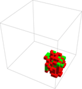
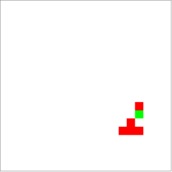
To display the results of the data, I defined two functions, one for displaying the entire 3D grid, and one for displaying a cross-section of it. When neurons are resting, they are transparent or white. When they are refractory, they are transparent in 3D and gray in 2D. Excitatory cells that are firing are red, and inhibitory cells that are firing are green.
Displays the 2D cross-section:
In[]:=
display2D[cells_]:=ArrayPlot[cells,ColorFunction->(Which[#==0,White,#==1,Red,#==2,Green,#<0,Gray]&),ColorFunctionScaling->False]
Displays the 3D grid:
In[]:=
display3D[cells_]:=ArrayPlot3D[cells,ColorFunction->(Which[#==0,Transparent,#==1,Red,#==2,Green,#<0,Transparent]&),ColorFunctionScaling->False]
Running of simulation
Running of simulation
To run the simulation, I created the initial conditions for the cell automata, including the initial grid of cells, the list of excitatory neurons, the list of neighbors, and the initial firing cells. Then, I repeatedly applied the updateCells function for a certain number of frames.
Runs the simulation with the given parameters:
In[]:=
runSimulation[dimensions_,inhibitoryProportion_,excitationProbability_,threshold_,initialFiringNum_,refractoryPeriod_,runTime_]:=Module[{initCells=createCells[dimensions],excitatoryNeurons=chooseExcitatory[dimensions,inhibitoryProportion],neighbors=createConnections[dimensions],initialFiring,initialStimulus},initialFiring=initiateFiring[initialFiringNum,excitatoryNeurons,initCells];initialStimulus=initialFiring[[1]];initCells=initialFiring[[2]];NestList[updateCells,{initCells,initialStimulus,{},{},excitatoryNeurons,excitationProbability,refractoryPeriod,0,False,dimensions,threshold,neighbors},runTime]]
Simulation of the Results
Simulation of the Results
Shown are the results of the simulation using 20% inhibitory neurons and an excitation probability of 90%. To display the results, I created the visual representation of the cells (3D and 2D) and the graph of firing neurons over time.
Runs the simulation with 20% inhibitory neurons and a 90% excitation probability:
In[]:=
stages=runSimulation[{20,20,20},0.2,0.9,1,1,3,100];
In[]:=
frames=stages[[All,1]];
Creates the 3D animation and the 2D animation of a cross-section:
In[]:=
ListAnimate[display3D/@frames]
Out[]=
Displays a cross section of the grid:
In[]:=
framesCrossSection=stages[[All,1]][[All,10]];
In[]:=
ListAnimate[display2D/@framesCrossSection]
Out[]=
This graph shows the number of firing neurons at each time step. The behavior of the graph shows an exponential growth of the number of firing neurons and then settling into an oscillatory pattern.
Plots the number of action potentials of the neurons over time
Observations of the Graphs
Observations of the Graphs
The following graphs show the number of action potentials over time for all the neurons.
When using a model of 8000 neurons, 20% inhibitory, and an excitation probability of 40%, the number of firing neurons first increases rapidly due to all the cells being in the resting stage. Then, it fluctuates about a value of around 700 neurons. Unlike the previous example, the activity fluctuates randomly instead of having a more defined periodicity.
Plots 200 steps of the simulation:
Next, I represented a constant stimulus by refiring all 100 initial neurons every 30 frames. The parameters used was a 20% inhibitory proportion and 27% excitation probability. When considering a simulation where all the initial excitatory neurons refire at regular intervals, the activity is much more rapid, which reflects knowledge on how brain activity increases during stimulation.
Graph of the Number of Firing Cells Over Time:
For certain parameters, I observed behavior with a long period of oscillation. For example, using an inhibitory proportion of 22% and an excitation probability of 32%, the activity reflected a sinusoid with a longer period. The significance of this long period is that brain waves come in different frequencies that reflect different functions (Trafton, 2015).
Plots 100 steps of the simulation:
Comparison with electroencephalograms (EEG)
Comparison with electroencephalograms (EEG)
When comparing the results of the graphs with EEGs, the results look similar. Both have oscillatory patterns (“brain waves”) as well as random fluctuations. Brain waves are important in the brain because they play a role in memory formation, learning, neural coordination, etc (Trafton, 2015). It’s not clear how brain waves form, but my findings could show that even simple neural models can create these patterns.
(Electroencephalography, 2026).
Variation of the Parameters
Variation of the Parameters
Each simulation of the cellular automata relies on initial conditions. By varying the parameters of the simulation, I can observe the different kinds of behavior produced. The parameters that I used were the proportion of inhibitory neurons and the excitation probability. The proportion of inhibitory neuron is an important part of the experiment because the balance between excitatory and inhibitory neurons is very important. For example, epilepsy is associated with lower levels of inhibition (Žiburkus et al., 2013). Similarly, the excitation probability is the probability that a neuron is able to be activated, so modifying that variable will also reflect higher neural excitation.
Runs the trials with the parameters of inhibitory proportion (a) and excitation probability (b):
For each pair of possible parameters, I measured the average number of firing neurons in the last 50 steps of the cellular automata. The results show that at a small proportion of inhibitory neurons and high excitation probabilities, brain activity is higher. These irregularities, which reflect disorders like epilepsy, are associated with increased excitation in the brain (Žiburkus et al., 2013). This is reflected by my model because at lower levels of inhibitory neurons, the brain activity was much higher. Empirically, this is associated with epileptic seizures and can be visualized in the below phase diagrams (NIH, n.d.).
In the graph shown below, I simulated with an inhibitory proportion from 0 to 0.8 with a step size of 0.01 and with the excitation probability from 0.2 to 1 with a step size of 0.01.
Goes through each possible pair of parameters and graphs the average number of firing neurons in the last 50 time steps:
Next, I classified the behavior of the neurons for each condition into two types: death (all cell’s eventually stop firing) or stable (cells maintain a somewhat stable population). For the death (blue) cases, I measured the time it took for the cells to die out. Darker colors are cases where it took longer for all neurons to die out. For the stable (yellow) cases, I measured how much they can be approximated by a sinusoidal function. Darker colors represent behavior that is more regular, as it can be approximated better by a periodic function.
Classifies the two types of behavior and then calculates the appropriate value.
The results show that high excitation probabilities and low numbers of inhibitory neurons result in highly oscillatory patterns (the dark brown colors). These highly oscillatory firing patterns are associated with the mechanisms for diseases such as epilepsy (Shao et al., 2021). For the death cases, higher proportions of inhibitory neurons and a smaller excitation probability result in the cells dying out faster.
Conclusion
Conclusion
In this project, I used cellular automata to model neural firing patterns. I defined a set of simple rules based on neural connections and studied the emergent behavior from these rules. When measuring the brain activity of the neurons, it showed behaviors similar to those in EEGs, indicating that the model is capable of displaying accurate behavior that reflects empirical data.
Additionally, when varying the parameters used in the simulation, I found that it was consistent with scientific knowledge on neurological conditions. While my model was used on a small scale, it simplified the computation necessary to simulate neural firing. I constructed phase diagrams that visualized the changes in the time series data from the automaton as different parameters changed. This allowed me to observe trends in the overall long-term behavior of my automaton. Notably, lower numbers of inhibitory cells and a higher probability of excitation resulted in highly regular patterns, reflecting scientific knowledge on neurological disorders.
Future Directions
Future Directions
To improve this project, more accurate methods could be used to simulate neural firing activity. First, the model was implemented with a small number of neurons and a small number of connections. Making the model more interconnected and using a larger number of neurons will help show more accurate behavior. Second, the shape of the brain was a cube, which doesn’t accurately reflect how cells in the brain are organized. A model that accounts for the organization of cells in the brain will be more accurate. Also, experimenting with different shapes of the brain, such as having two hemispheres of the brain can be used to show how the two hemispheres of the brain interact. Third, the analysis of the brain activity with the EEGs was not quantitative, so using statistical tests that compare the two will better support the connection between the simulated brain activity and EEGs. Fourth, the classification of the behavior for each set of parameters did not account for individual details of the graphs and grouped them into broad classes. Using a more specific classification method would better show which set of parameters are associated with certain types of brain behavior.
Acknowledgements
Acknowledgements
Thank you to William Choi-Kim for mentoring me. I am grateful for his guidance on my project. I also would like to thank the WSRP program directors for this amazing experience. I really enjoyed WSRP and learned a lot. I would also like to thank Stephen Wolfram for his guidance and ideation.
References
References
◼
Electroencephalography. (2026). In Wikipedia. https://en.wikipedia.org/w/index.php?title=Electroencephalography&oldid=1363251273
◼
Kuriyama, R., Akira, K., Green, L., Herrera, B., Dai, K., Iura, M., Gouaillardet, G., Terasawa, A., Kobayashi, T., Igarashi, J., Arkhipov, A., & Yamazaki, T. (2025). Microscopic-level mouse whole cortex simulation composed of 9 million biophysical neurons and 26 billion synapses on the supercomputer Fugaku. Proceedings of the International Conference for High Performance Computing, Networking, Storage and Analysis, 2158–2171. https://doi.org/10.1145/3712285.3759819
◼
NIH. (n.d.). Epilepsy and seizures. Retrieved July 9, 2026, from https://www.ninds.nih.gov/health-information/disorders/epilepsy-and-seizures
◼
Shao, J., Liu, Y., Gao, D., Tu, J., & Yang, F. (2021). Neural burst firing and its roles in mental and neurological disorders. Frontiers in Cellular Neuroscience, 15, 741292. https://doi.org/10.3389/fncel.2021.741292
◼
Sukenik, N., Vinogradov, O., Weinreb, E., Segal, M., Levina, A., & Moses, E. (2021). Neuronal circuits overcome imbalance in excitation and inhibition by adjusting connection numbers. Proceedings of the National Academy of Sciences, 118(12), e2018459118. https://doi.org/10.1073/pnas.2018459118
◼
Trafton, A. (2015, February 23). How brain waves guide memory formation. MIT News | Massachusetts Institute of Technology. https://news.mit.edu/2015/brain-waves-guide-memory-formation-0223
◼
Žiburkus, J., Cressman, J. R., & Schiff, S. J. (2013). Seizures as imbalanced up states: Excitatory and inhibitory conductances during seizure-like events. Journal of Neurophysiology, 109(5), 1296–1306. https://doi.org/10.1152/jn.00232.2012
CITE THIS NOTEBOOK
CITE THIS NOTEBOOK
Modeling neural firing using cellular automata
by Minghao Guo
Wolfram Community, STAFF PICKS, July 9, 2026
https://community.wolfram.com/t/27195
by Minghao Guo
Wolfram Community, STAFF PICKS, July 9, 2026
https://community.wolfram.com/t/27195