FOMC day
FOMC day
This notebook takes a look at stock market data which is believed to be transaction by transaction data scraped from the NASDAQ website’s realtime quote section for the SPY ETF. By the volumes it does not appear to be the total volume of shares traded on the selected day, 4 May 2022. This was the day the the Federal Reserve Open Market Committee announced a 0.5% interest rate increase at 14:00 Eastern Time. The data are embedded into the notebook as a ByteArray of a zipped file and extracted below.
In[]:=
byteString=FromCharacterCodeNormalByteArray;may4=ImportString[byteString,{"ZIP","spy04May2022.wl"}];
The dataset consists of 250257 sequential transactions.
In[]:=
Length@may4
Out[]=
250257
The data format is {dateObject, price, volume}. dateObject has a resolution of only 1 second, so it cannot be used for ordering the data.
In[]:=
may4[[1]]
Out[]=
,417.08,200
Below the data are converted to minute data with {dateObject, open, high, low, close, volume} for each minute. The minute volatility is calculated as Log[high/low] for each minute. A simple intraday volatility measure
In[]:=
minuteData={#[[1]][[1]],First[#[[All,2]]],Max[#[[All,2]]],Min[#[[All,2]]],Last[#[[All,2]]],Total[#[[All,3]]]}&/@Split[may4,DateValue[#1[[1]],"Minute"]==DateValue[#2[[1]],"Minute"]&];
In[]:=
GraphicsColumnDateListPlotminuteData[[All,{1,5}]],,DateListPlot{#1,Log[#3/#4]}&@@@minuteData,
Out[]=
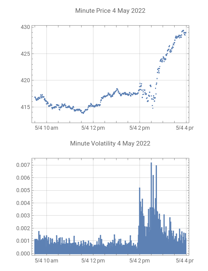
The graphs above show a dramatic increase in volatility after the FOMC announcement. The rest of this notebook explores the overall tail behavior of the data and also looks at the before and after time frames to look for differences. The data is split into before and after timeframes:
In[]:=
may4a=Take[may4,92077];may4b=Drop[may4,92077];may4a[[-1]]may4b[[1]]
Out[]=
,418.205,100
Out[]=
,418.14,100
First the logarithmic returns are calculated for the whole day’s data. More than 98,000 sequential transaction price changes are zero.
In[]:=
lr=Differences[Log[may4[[All,2]]]];Length[lr]Count[lr,0.]
Out[]=
250256
Out[]=
98878
Here is the histogram showing the large spike near zero. This is not like any continuous statistical distribution, but there should be enough data points to examine the tail behavior of the data.
In[]:=
Histogram[lr,Automatic,"PDF",PlotRange->All]
Out[]=
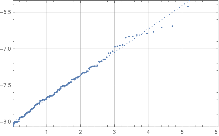
Here the 300 most extreme positive and negative returns are selected and tested for power tail behavior by taking the Log[tail] and comparing it to an exponential distribution, then estimating the power tail exponent. -7.5 log price change amounts to about a change in average price of 23 cents.
tail=Take[Sort[Abs[lr]],-300];qqp=QuantilePlotLog[tail],ExponentialDistribution[1],Method{"ReferenceLineMethod""Fit"},tailSlope=Cases[Cases[qqp,Rule[Epilog,x_]x,∞],Line[xx_]xx,∞];
Out[]=
In[]:=
Mean[may4[[All,2]]]Exp[-7.5]
Out[]=
0.232651
The tail exponent calculated from the slop of the fit reference line.
In[]:=
(#1/#2&@@@Differences[tailSlope[[1]]])[[1]]
Out[]=
3.12017
The tail exponent calculated by fitting adjusted log tail to an exponential distribution.
In[]:=
fit1=EstimatedDistribution[Log[Select[tail,#>Min[tail]&]]-Log[Min[tail]],ExponentialDistribution[α]]
Out[]=
ExponentialDistribution[2.6453]
The tail exponent calculated from a point on the empirical characteristic function, consistent with an exponential distribution.
In[]:=
powerTailAlpha[data_]:=With[{mn=Min[data]},Cot[Arg[Mean[Exp[I(Log[Select[data,#>mn&]]-Log[mn])t]]-1/2]/2]t/.t1024$MachineEpsilon];
In[]:=
fit2=powerTailAlpha[tail]fit1[[1]]-fit2
Out[]=
2.6453
Out[]=
4.44089×
-16
10
The tail analysis is repeated below for the data before the FOMC announcement.
In[]:=
lr=Differences[Log[may4a[[All,2]]]];
In[]:=
Length[lr]
Out[]=
92076
The fit here is not so clear because the data are showing some step like changes because prices usually have maximum resolution in the dataset of one cent.
tail=Take[Sort[Abs[lr]],-100];qqp=QuantilePlotLog[tail],ExponentialDistribution[1],tailSlope=Cases[Cases[qqp,Rule[Epilog,x_]x,∞],Line[xx_]xx,∞];
Out[]=
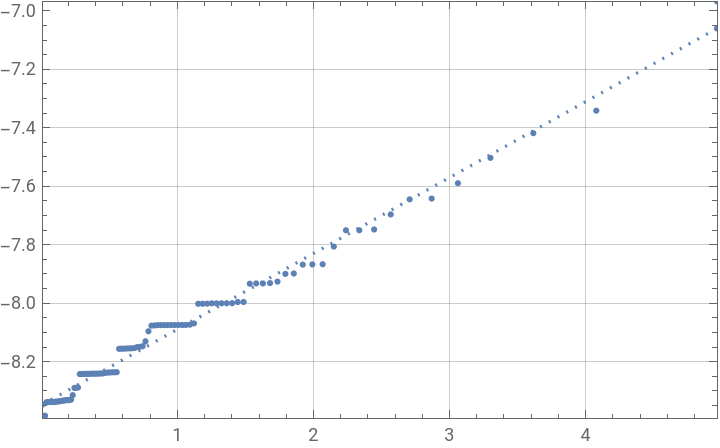
The tail exponents for the morning data appear to by higher, i.e. the return distribution tails may be lighter with lower volatility.
In[]:=
(#1/#2&@@@Differences[tailSlope[[1]]])[[1]]
Out[]=
3.85371
In[]:=
fit1=EstimatedDistribution[Log[Select[tail,#>Min[tail]&]]-Log[Min[tail]],ExponentialDistribution[α]]
Out[]=
ExponentialDistribution[3.28316]
Data after the FOMC announcement, may4b. There are more data points here.
The power tail exponent appears to be a little lower after the announcement .
Data reliability
Data reliability
The quality of this dataset is not really known. The hundred largest price magnitude jumps of the day.
Here the price jumps larger than 30 cents are selected.
There are 13 of these jumps selected both positive and negative. The code below will print out all of the local prices with the jump occurring at index 50 on the graph and the whole graph showing 49 transactions before the jump transaction and 150 prices after. Only three of the graphs are shown below to conserve space.
The first graph below looks like a sudden bona fide change in price--the price dramatically changes and subsequent prices are impacted by the jump. The second graph, however, looks more like a pricing error that was not noticed by the market. The price dramatically changed then reversed itself with no impact on subsequent prices. This would represent two tail events one negative and the other positive. If these jumps represent bad data it will impact tail analysis. The third graph looks like a big jump which seemed to be recovering, but the subsequent market prices were affected and there was increasing volatility after the event, so this appears to be a real event.
The first graph below looks like a sudden bona fide change in price--the price dramatically changes and subsequent prices are impacted by the jump. The second graph, however, looks more like a pricing error that was not noticed by the market. The price dramatically changed then reversed itself with no impact on subsequent prices. This would represent two tail events one negative and the other positive. If these jumps represent bad data it will impact tail analysis. The third graph looks like a big jump which seemed to be recovering, but the subsequent market prices were affected and there was increasing volatility after the event, so this appears to be a real event.
These are the transaction volumes with each spike. The spikes do not seem to be associated with any large block trade.
Conclusion
Conclusion
The notebook examines some high frequency data which is probably of reasonable quality to look at a natural volatility experiment on a day where there is a large jump in market volatility due to the FOMC announcement. More of these days need to be analyzed, to come to any solid conclusions about tail exponent in market returns with respect to volatility. It would be very helpful to have a curated data base in the Wolfram Data Repository which extended over many years.