Paclet Installation
Paclet Installation
Theory
Theory
In a previous post, we demonstrated the Variational Quantum Linear Solver (VQLS), a hybrid quantum-classical technique designed to solve Quantum Linear Systems Problems (QLSP). Simply put, it finds linear solutions for equations of the form ””.
A.x=b
We propose an Multiplexer–Based Variational Quantum Linear Solver (MB-VQLS). The primary distinctions between MB–VQLS and a conventional VQLS lie in two key aspects:
◼
The controlled implementation of the matrix through a multiplexer, enabling the accurate representation of the operation within the quantum circuit.
A
A.x
◼
The solution to the linear system is encoded directly in the amplitudes of the resultant quantum state.
This approach simplifies the standard VQLS process of using multiple circuits for the real-imaginary decomposition of the solution and the termwise (term-by-term) computation in quantum circuits. A detailed step-by-step for this implementation is provided in this notebook.
To summarize the problem statement, given:
◼
Problem vector b: Normalized quantum state
|b〉.
◼
Problem matrix A: x matrix such that where ϵ and
n
2
n
2
A=
L-1
∑
0
c
l
A
l
c
l
||A||<=1
We pursue to prepare:
◼
A quantum statesuch that with
|x〉
A|x〉=|〉
ψ
=1
b
ψ
2
For this, we will obtain approximated states through a variational quantum circuit (ω):
|x(ω)〉
V
|x(ω)〉=V(ω)|0〉
And we will be minimizing a cost function with parameters to reach our goal:
ω={,,...}
ω
0
ω
1
f(ω)=1-
b
ψ(ω)
2
Further steps will show that we can avoid some and restrictions using their normalization terms. This would help us finding solutions for any system.
|b〉
A
In the following examples we won’t limit to solve simple Pauli system problems as previous posts, we will start right away with real and complex random vectors and random problem matrices.
b
A
A.x Operation Circuit Representation
A.x
For this section, we will follow the guide already published by the Wolfram Quantum Computation Framework Team.
Considering an x A matrix and an -element vector x, we look to compute the operation with a quantum circuit using as a controlled operation.
n
n
n
A.x
A
Given:
In[]:=
x=RandomComplex[{-1-1*I,+1+1*I},4]
Out[]=
{-0.347991+0.931491,-0.0392888-0.0284354,0.103762+0.831308,-0.489936+0.6389}
In[]:=
a=RandomReal[{-1,1},{4,4}];a//MatrixForm
Out[]//MatrixForm=
0.798301 | 0.574044 | 0.915333 | 0.202758 |
-0.917779 | 0.00718937 | -0.695192 | 0.127807 |
0.317395 | -0.307586 | 0.0114712 | -0.391997 |
-0.109567 | 0.557948 | -0.228003 | -0.486929 |
We proceed to generate a quantum operator and decompose it in Pauli Matrices such that
A
A=:
c
j
A
j
In[]:=
A=QuantumOperator[a];
In[]:=
pauliDecompose=A["PauliDecompose"]
Out[]=
XX-0.227397+0.,XY0.+0.174982,XZ0.136743+0.,XI0.479621+0.,YX0.-0.0188202,YY-0.273992+0.,YZ0.+0.25702,YI0.+0.0419493,ZX0.0690661+0.,ZY0.+0.413954,ZZ0.0731779+0.,ZI0.320237+0.,IX-0.240934+0.,IY0.+0.331957,IZ0.322378+0.,II0.0825082+0.
In order to implement the controlled A gates, we will turn the Pauli matrices as targets into a Multiplexer and the controlled qubits would be evaluated by a state:
c
In[]:=
multiplexer=QuantumCircuitOperator["Multiplexer"@@Keys[pauliDecompose]];
In[]:=
ancillary=QuantumStateSqrt@Values[pauliDecompose],"Label"->"";
c
Finally, we would let our vector be evaluated by the multiplexer in our citcuit:
x
In[]:=
productCircuit=QuantumCircuitOperatorancillary,QuantumState[x,"Label"->"x"]->{5,6},multiplexer,;
†
ancillary["Conjugate"]
In[]:=
productCircuit["Diagram",ImageSize->Full]
Out[]=
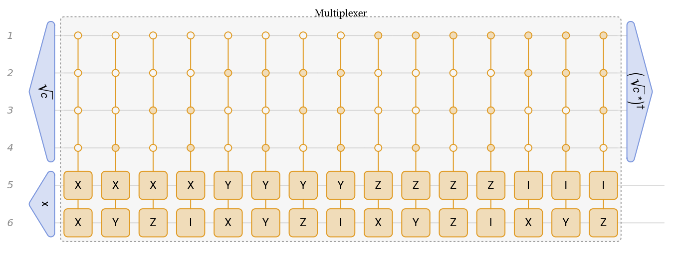
Evaluate our circuit and check the amplitudes of the resultant state:
In[]:=
productCircuit[]["AmplitudesList"]
Out[]=
{-0.304717+1.61775,0.184345-1.35137,0.0948776+0.0634864,0.231113-0.618566}
The result correspond to the equivalent classical operation:
In[]:=
a.x
Out[]=
{-0.304717+1.61775,0.184345-1.35137,0.0948776+0.0634864,0.231113-0.618566}
Quantum Linear Solver Implementation
Quantum Linear Solver Implementation
Now that we learned how to compute the product of a matrix and vector using a Quantum Circuit, we have a better understanding on how to implement our new variational quantum linear solver.
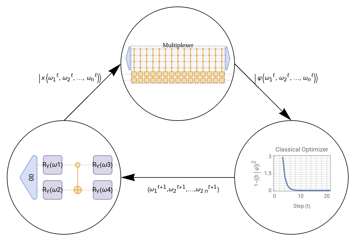
Given a problem vector and an problem matrix, the basic steps are:
b
A
◼
Start with a variational circuit ansatz or state ansatz
V()
ω
i
x()=V()|0〉
ω
i
ω
i
◼
Apply the multiplexer such that we perform and obtain resultant state
A.x()
ω
i
ψ()
ω
i
◼
Use state as input for the optimizer with the cost function to obtain new parameters
ψ()
ω
i
f(ω)=1-
b
ψ(ω)
2
ω
j
◼
Use new parameters with the variational circuit or state ansatz
ω
j
V()
ω
i
x()
ω
j
◼
Repeat the process until you obtain
f()=1-=0
ω
opt
b
ψ()
ω
opt
2
Initial problem setup
Initial problem setup
Multiplexer implementation
Multiplexer implementation
For this section we need to repeat what is stated in “ Operation Circuit Representation“ section.
A.x
First, we need to decompose in Pauli matrices such that =∑ :
A
A
c
i
A
i
In[]:=
pauliDecompose=QuantumOperator[matrixA/normA]["PauliDecompose"];
In[]:=
pauliDecompose
Out[]=
XX0.238307+0.,XY0.-0.0171748,XZ0.153066+0.,XI0.255368+0.,YX0.+0.0221491,YY0.167908+0.,YZ0.+0.0149763,YI0.+0.0309613,ZX0.0582089+0.,ZY0.-0.0975743,ZZ-0.0302903+0.,ZI0.00164333+0.,IX0.249554+0.,IY0.+0.0029762,IZ-0.109616+0.,II0.192193+0.
Next, implement the multiplexer:
multiplexer=QuantumCircuitOperator["Multiplexer"@@Keys[pauliDecompose]];
In[]:=
ancillary=QuantumStateSqrt@Values[pauliDecompose],"Label"->"
c
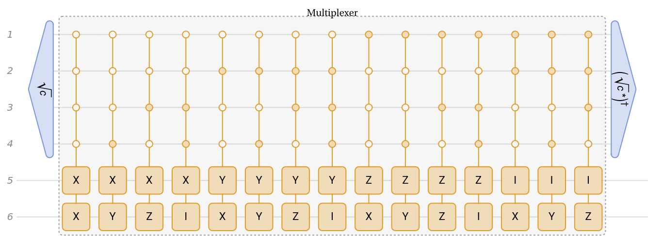
";We obtain the first section of the variational circuit for the VQLS:
In[]:=
CircuitA=QuantumCircuitOperatorancillary,multiplexer,;
†
(ancillary["Conjugate"])
In[]:=
CircuitA["Diagram",ImageSize->Full]
Out[]=
General Symbolic Ansatz
General Symbolic Ansatz
Define a general state ansatz for 4-qubits with real amplitudes:
Finally we implement the circuit and the correspondent state:
Wolfram Quantum Framework quantum states (and measurements) keep the parameters defined in previously used circuits, so it would be optimum to work with the resultant state:
Optimization
Optimization
In order to correct our result, we need to find the global phase and apply it once our calculation is done.
Optimization using NMinimize
Optimization using NMinimize
Let’s optimize the cost function using NMinimize:
As previously stated, while the probability distributions match, the amplitudes do not necessarily align:
We can verify our result:
Optimization using Quantum Natural Gradient Descent
Optimization using Quantum Natural Gradient Descent
As explained in a previous example, we can optimize using QuantumNaturalGradientDescent calculating their correspondent Fubini-Study metric tensor:
Check the evolution of the minimization using a simple plot:
We can verify that the minimization approaches to 0.
As previously stated, while the probability distributions match, the amplitudes do not necessarily align:
We can verify our result approximation:
QuantumLinearSolve Function
QuantumLinearSolve Function
The QuantumLinearSolve function is a new addition to the Wolfram Quantum Framework. It simplifies the process of solving linear systems with hybrid classical-quantum algorithms by condensing previous code into a single function.
Use QuantumLinearSolve function to solve the linear system. This function will implement the necessary multiplexer and determine the optimal general ansatz state to solve the QLSP:
Finally compare the results:
Our result demonstrate a high degree of approximation accuracy:
Properties
Properties
It is possible to ask for every element used in the implementation indicating a property as third input:
Scope & Method
Scope & Method
It is also possible to add multiple options for the minimization such as AccuracyGoal and PrecisionGoal:
You can use multiple methods for the optimization which will display a progression plot:
More about the properties, methods and functionalities of QuantumLinearSolve in the following documentation page:
https://resources.wolframcloud.com/PacletRepository/resources/Wolfram/QuantumFramework/tutorial/ExampleRepositoryFunctions.html
https://resources.wolframcloud.com/PacletRepository/resources/Wolfram/QuantumFramework/tutorial/ExampleRepositoryFunctions.html
References
References
◼
Mads Bahrami (2024). Compute the Product of a Matrix and Vector using a Quantum Circuit. Wolfram Example Repository. https://resources.wolframcloud.com/ExampleRepository/resources/Coherent-applying-of-a-matrix-on-a-vector/
◼
Bravo-Prieto, C., LaRose, R., Cerezo, M., Subasi, Y., Cincio, L., & Coles, P. J. (2019). Variational Quantum Linear Solver. arXiv. https://doi.org/10.48550/ARXIV.1909.05820
◼
Mari, A. Variational Quantum Linear Solver. PennyLane Demos. https://pennylane.ai/qml/demos/tutorial_coherent_vqls/
CITE THIS NOTEBOOK
CITE THIS NOTEBOOK
Multiplexer-based variational quantum linear solver
by Sebastian Rodriguez
Wolfram Community, STAFF PICKS, August 22, 2024
https://community.wolfram.com/groups/-/m/t/3253903
by Sebastian Rodriguez
Wolfram Community, STAFF PICKS, August 22, 2024
https://community.wolfram.com/groups/-/m/t/3253903