ABSTRACT(original article): We present the solution of six problems drawn from the chemical engineering and applied mathematics fields of study. These problems are solved using the arc-length continuation method. Among a large number of examples, we have chosen to treat the following case studies because they illustrate basic concepts such as solution multiplicity when dealing with systems of nonlinear algebraic equations or boundary value problems: 1) Plotting an ∞-shaped curve called the Bernoulli’s Lemniscate; 2) Computing the Joule-Thomson inversion curve for a pure gas using the Soave-Redlich-Kwong cubic equation of state; 3) Predicting the Compressibility Factor and Molar Volume versus the Reduced Temperature; 4) Determining region where steady-state multiplicity is observed in a continuous stirred-tank reactor (CSTR) with multiple reactions and heat effects; 5) Finding the steady-state temperature and conversion of a Propylene Glycol Reactor; and 6) Investigating the Frank–Kamenetskii problem arising in the self-heating of a reactive solid. Reader should be advised that problem 1 may seem slightly mathematical in nature. However, case studies 2–6 could be very useful to instructors involved in teaching not only numerical methods but also chemical thermodynamics and chemical reaction engineering. For one of the above listed case studies, we unveil the MATLAB© code, that we have employed, in the Appendix. In addition, we will emphasize on the versatility of this mathematical software through the extensive usage of the built-in command fsolve, for the presently undertaken computations. Finally, we conclude this paper by sharing our experience teaching this subject to graduate students at King Fahd University of Petroleum & Minerals. CITATION (original article): U. Al-Mubaiyedh and H. Binous, Teaching arc-length continuation in the chemical engineering graduate program using MATLAB©, Comput Appl Eng Educ. 2018; 26: 1033–1049. DOI: https://doi.org/10.1002/cae.21954
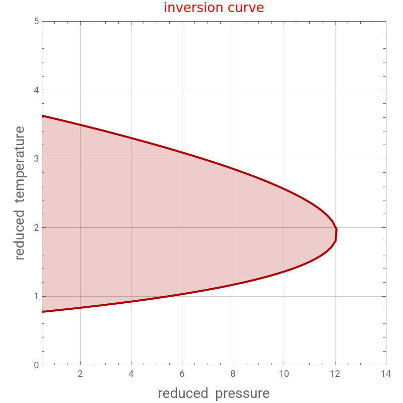
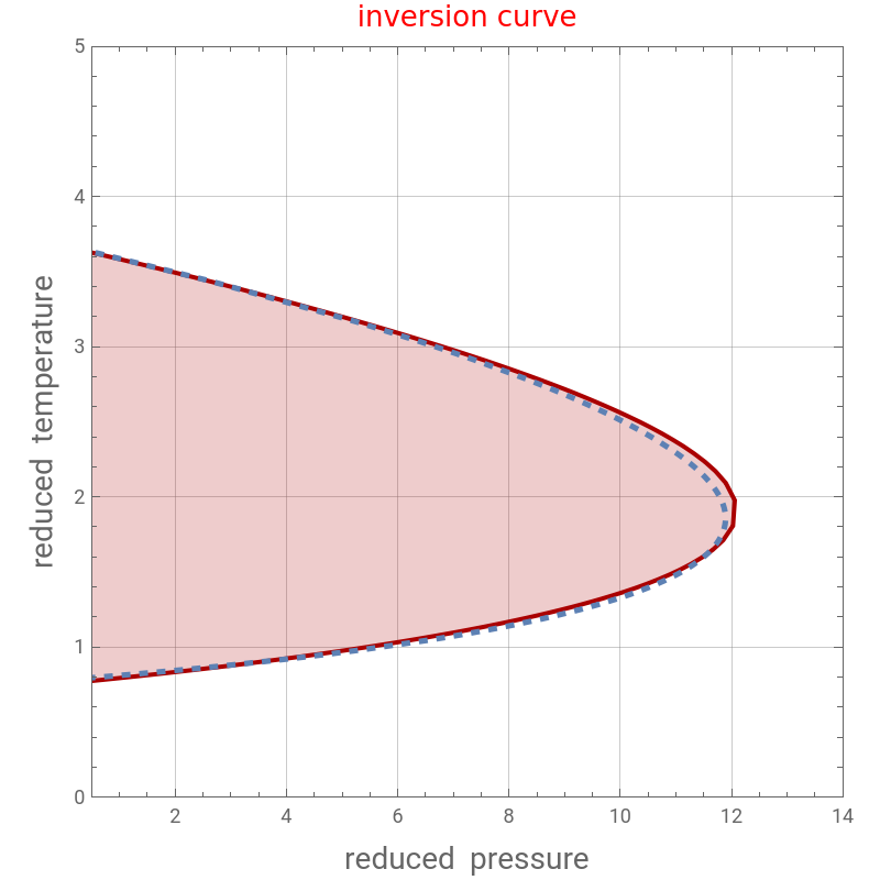
Throttling a real gas can sometimes result in a temperature decrease. If such is the case, the Joule–Thomson coefficient is positive. This coefficient can be written as:, where is the universal gas constant, is the constant-pressure heat capacity and is the compressibility factor. In order to estimate the value of , the Soave–Redlich–Kwong (SRK) equations of state is selected. We use the arc-length continuation to compute the Joule–Thomson inversion curve (i.e. the loci of the points, in the - plane, where ). Here, following Ref. 1, we choose propylene, but the program can be modified for any other pure component. A point inside the colored area indicates that the value of the Joule–Thomson coefficient is positive; otherwise . The inversion curve and colored region are both indicated in red (for the SRK EoS).Finally, we compare our results with the fit based on Miller’s work (see Ref. 2).
μ=
∂T
∂P
H
μ=P
R
2
T
c
P
∂Z
∂T
P
R
c
P
Z
μ
P
r
T
r
μ=0
μ<0
Approach based on arc-length continuation and NDSolve
Propylene data
Tc=365.6;Pc=46.65;ω=0.14;
Gas constant
R=8.314;
The SRK cubic equation of state
m=0.480+1.574ω-0.176ω^2;a=(1+m(1-Tre^0.5))^2;A=0.42748aPre/Tre^2;B=0.08664Pre/Tre;eqZ=Z^3-Z^2+Z(A-B^2-B)-AB0;
Gas-phase compressibility factor
Zv1=Z/.Solve[eqZ,Z][[1]];derv1=D[Zv1,Tre];(**)
∂Z
∂T
P
Setting μ=0
eq1=(Re[derv1]0)/.TreTre[s]/.PrePre[s];eq2=Tre'[s]^2+Pre'[s]^21;(*auxiliaryequation*)
Initial conditions
init1=Tre[0](Tre/.FindRoot[(derv1/.Pre5)0,{Tre,3.5}]//Chop);init2=Pre[0]5;
Solution using NDSolve
sol=Quiet@NDSolve[{eq1,eq2,init1,init2,Tre'[0]-0.001,Pre'[0]0.001},{Pre,Tre},{s,-100,1000},Method{"EquationSimplification""Residual"},AccuracyGoal3];
Bounds for the qrc-length s
Ubound=sol[[1,1,2]][[1,1]][[2]];Lbound=-10;
In[]:=
tbl=Table[Flatten[Evaluate[{Pre[s],Tre[s]}/.sol]],{s,Lbound,Ubound,0.2}];s1=ListPlot[tbl,JoinedTrue,AspectRatio1,GridLinesAutomatic,FrameTrue,PlotRange{{0.5,14},{0,5}},PlotStyle{Thick,Darker@Red},FrameLabel->{Style["reduced pressure",14],Style["reduced temperature",14]},ImageSize{400,400},FillingAxis,PlotLabelStyle[Text["inversion curve"],Red,13]]
Out[]=
In[]:=
tbl2=Table[Flatten[Evaluate[{Tre[s],Pre[s]}/.sol]],{s,Lbound,Ubound,0.05}];
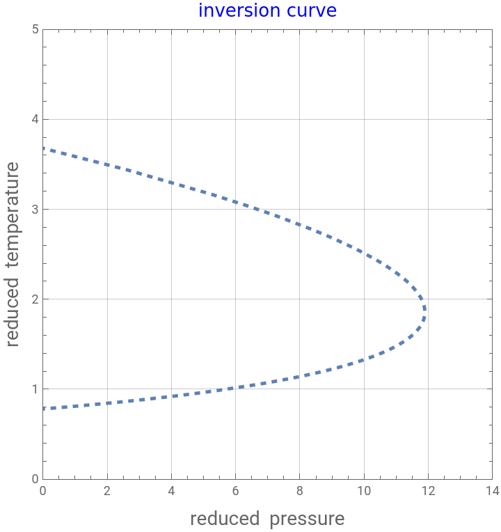
Following the treatment of Miller (see Ref. 2), we fit the inversion curve data (see the dashed blue line in Figure below) using the following empirical equation : =α-β/-γ and NonlinearModelFit
P
r
T
r
2
T
r
In[]:=
opt=NonlinearModelFit[tbl2,α-β/x-γx^2,{α,β,γ},x]
Out[]=
FittedModel
In[]:=
Normal[opt]
Out[]=
30.3488--1.784
22.8497
x
2
x
In[]:=
opt["BestFitParameters"]
Out[]=
{α30.3488,β22.8497,γ1.784}
In[]:=
opt["RSquared"]
Out[]=
0.998822
In[]:=
p1=ParametricPlot[{Normal[opt],x},{x,0,13},PlotStyle->{Thickness[0.0075],Dashed},Frame->True,PlotRange->{{0,14},{0,5}},AspectRatio->1,GridLines->Automatic,FrameLabel->{Style["reduced pressure",14],Style["reduced temperature",14]},PlotLabelStyle[Text["inversion curve"],Blue,13]]
Out[]=
Miller’s fit and the exact SRK solution are superimposed on the same plot
In[]:=
Show[s1,p1]
Out[]=
References
References
◼
[1] U. Al-Mubaiyedh and H. Binous, Teaching arc-length continuation in the chemical engineering graduate program using MATLAB©, Comput Appl Eng Educ. 2018; 26: 1033–1049. https://doi.org/10.1002/cae.21954
◼
[2] G. Miller, Joule-Thomson inversion curve, corresponding states, and simpler equations of state, Ind. Eng. Chem. Fundam., 9 (1970), pp. 585–589.
CITE THIS NOTEBOOK
CITE THIS NOTEBOOK
Computing the Joule-Thomson inversion curve for a pure gas using the Soave-Redlich-Kwong
by Housam Binous and Ahmed Bellagi
Wolfram Community, STAFF PICKS, December 23, 2024
https://community.wolfram.com/groups/-/m/t/3342780
by Housam Binous and Ahmed Bellagi
Wolfram Community, STAFF PICKS, December 23, 2024
https://community.wolfram.com/groups/-/m/t/3342780