Introduction
Introduction
Mathematica has long supported the traditional colorspaces like RGBColor (corresponding to an additive color model, as used in screen displays), CMYKColor (corresponding to an subtractive color model, as used in printing), and Hue (the system implementation of hue-saturation-brightness, a.k.a. HSB). Relatively more recently, support for colorspaces like LABColor (corresponding to the CIE L*a*b* colorspace) and XYZColor (corresponding to the CIE XYZ colorspace) that closely model the perception of color in human vision was added.
In this notebook, I want to talk about various color-related functions I had implemented over the past few months, including a new approximation for the color-matching functions in XYZ space, as well as two recently devised colorspaces that have interesting properties.
New approximations to CIE color matching functions
New approximations to CIE color matching functions
The Commission internationale de l’éclairage (CIE, "International Commission on Illumination") is a non-profit organization based in Austria that, among other things, develops and publishes standards and procedures related to the subjects of light and lighting. This includes colorimetry, or the science of human color perception.
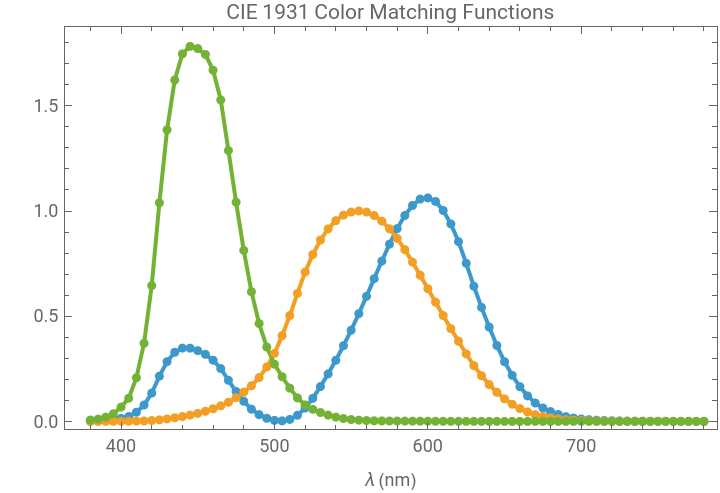
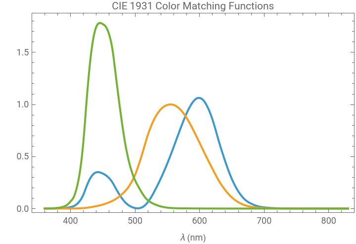
In 1931, CIE published standardized mathematical models of human color vision, based on the knowledge that human color vision is trichromatic. These models comprise the so-called "standard observer" of the CIE 1931 colorspace; among the results of this research (which came out of experiments done by Wright and Guild in the 1920s) are a set of so-called "color matching functions" (CMFs), denoted (λ), (λ), and (λ), that provide a standardized way to convert spectral radiance to a trichromatic color space. Crudely put, CMFs take a given wavelength of light as the argument, and produce tristimulus values; these are taken to be the components of the CIE XYZ colorspace, which can then be converted to other convenient color spaces like RGB.
x
y
z
The Wolfram Data Repository has the resource Selected CIE Colorimetric Tables that contains the data for the 1931 CMFs, among other things. Fetch the required data like so:
In[]:=
CIE1931Coarse=ResourceData["Selected CIE Colorimetric Tables","CIE1931"];
Dimensions[CIE1931Coarse]
Out[]=
{81,4}
The data included corresponds to the wavelengths 380 nm–780 nm, tabulated in 5 nm intervals; this spans the range of wavelengths for visible light:
MinMax[CIE1931Coarse[[All,1]]]
Out[]=
{380.,780.}
Differences[CIE1931Coarse[[All,1]]]//First
Out[]=
5.
We can now visualize the CMFs:
ListLinePlot{CIE1931Coarse[[All,{1,2}]],CIE1931Coarse[[All,{1,3}]],CIE1931Coarse[[All,{1,4}]]},AxesNone,FrameTrue,FrameLabel{"λ (nm)",""},
Out[]=


In[]:=
CIE1931Fine=Import["https://files.cie.co.at/CIE_xyz_1931_2deg.csv","CSV"];
Dimensions[CIE1931Fine]
Out[]=
{471,4}
MinMax[CIE1931Fine[[All,1]]]
Out[]=
{360,830}
Differences[CIE1931Fine[[All,1]]]//First
Out[]=
1
ListLinePlot{CIE1931Fine[[All,{1,2}]],CIE1931Fine[[All,{1,3}]],CIE1931Fine[[All,{1,4}]]},AxesNone,FrameTrue,FrameLabel{"λ (nm)",""},
Out[]=
As an example of how to use the tabulated CIE CMFs, we can construct InterpolatingFunction objects out of the tabulated CMFs (using Interpolation), like so:
{xb,yb,zb}=Interpolation/@{CIE1931Fine[[All,{1,2}]],CIE1931Fine[[All,{1,3}]],CIE1931Fine[[All,{1,4}]]}
Out[]=
InterpolatingFunction,InterpolatingFunction,InterpolatingFunction


With[{λ=589},Graphics[{XYZColor[xb[λ],yb[λ],zb[λ]],Disk[]},ImageSizeSmall]]
Out[]=
You can also visualize the entire visible spectrum, like so:
DensityPlot[λ,{λ,385,745},{y,0,50},AspectRatioAutomatic,ColorFunctionFunction[λ,XYZColor[xb[λ],yb[λ],zb[λ]]],ColorFunctionScalingFalse,FrameTicks{Automatic,None}]
Out[]=

The CMFs can also be used to generate the colors corresponding to electromagnetic radiation emitted by a blackbody, following Planck's law:
In[]:=
blackbodyColors[t_?NumericQ]:=With[{(*unnormalizedPlanckianspectralradiancefunction*)planck=1/((Exp[1.43877696*^7/(#t)]-1)#^5)&,(*BradfordD65->D50chromaticadaptationmatrix*)brad={{1.0478112,0.022886602,-0.050126976},{0.029542398,0.9904844,-0.017049096},{-0.0092344897,0.015043617,0.75213163}}},Apply[XYZColor,brad.Normalize[planck[CIE1931Fine[[All,1]]].CIE1931Fine[[All,{2,3,4}]],#[[2]]&]]]
DensityPlotT,{T,1000,10000},{y,0,1200},
Out[]=

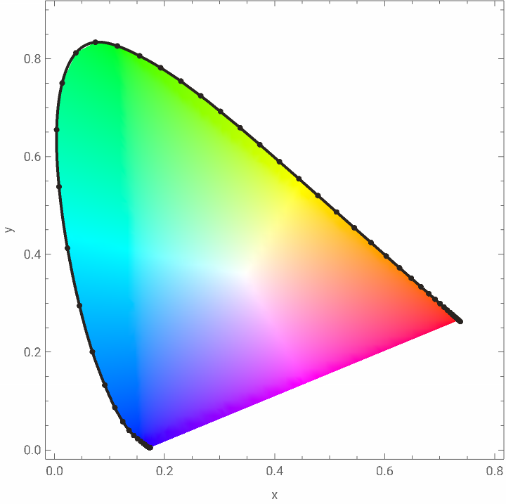
Finally, the CMFs are also used to define the boundary of the chromaticity diagram used for visualizing colors in colorspaces, as used in the function ChromaticityPlot:
Show[ChromaticityPlot[{},"CIE31"],ParametricPlot[{xb[λ],yb[λ]}/(xb[λ]+yb[λ]+zb[λ]),{λ,385,745},PlotStyleDirective[AbsoluteThickness[2],ColorData["Legacy","IvoryBlack"]]],ListPlot[CIE1931Coarse[[All,{2,3}]]/Total[CIE1931Coarse[[All,{2,3,4}]],{2}],PlotStyleDirective[AbsolutePointSize[4],ColorData["Legacy","IvoryBlack"]]]]
Out[]=
For some applications, keeping the tabulation of CMFs around can be unwieldy. Thus, there have been attempts to replace the tabulated CMFs with analytic approximations that are (relatively) simple to evaluate, and are reasonably accurate.
In[]:=
wssCMF[λ_]:=Module[{xf,yf,zf},xf={0.36263412,1.05593554,-0.2122116}.Exp[-MapThread[(λ-#1)Piecewise[{{#2,λ<#1},{#3,True}}]&,{{440.76797,599.44051,493.87482},{0.066588512,0.027633445,0.048888466},{0.020005468,0.032068622,0.039095442}}]^2/2];yf={0.82087906,0.28579841}.Exp[-MapThread[(λ-#1)Piecewise[{{#2,λ<#1},{#3,True}}]&,{{568.78966,530.87379},{0.021328878,0.061294726},{0.024693511,0.032178136}}]^2/2];zf={1.21649968,0.68126275}.Exp[-MapThread[(λ-#1)Piecewise[{{#2,λ<#1},{#3,True}}]&,{{436.96247,459.03433},{0.084453906,0.038519512},{0.027788061,0.072502761}}]^2/2];{xf,yf,zf}]
Another paper introducing approximants of the CIE CMFs is the paper of Puls. The Puls approximation uses scaled logistic/sigmoidal functions along with Gaussian functions; this is claimed to preserve chromaticity even outside the visible range. The following function implements the Puls approximation:
Note that in both implementations of the WSS and Puls approximants, I have used constants slightly different from the ones in the published papers. Instead of just directly taking the coefficients from the papers, I used the proposed models in FindFit along with NMinimize, using the 1 nm tabulation of the 1931 CMFs (defined earlier as CIE1931Fine) as the fitting data. (The function for the WSS approximant, in particular, was previously posted on Mathematica Stack Exchange; the Puls approximant is completely new. The resource function ResourceFunction["CIEColorMatchingFunctionValues"] also uses the WSS approximant.)
To facilitate comparison, here's a superfunction that allows you to choose between the two approximants, via a Method setting:
Test it out:
We can retry the example applications given earlier, but this time, we can replace the tabulated CMFs with the analytic approximations.
With that, here is a function for generating colors from the visible spectrum, using the analytic approximations implemented earlier:
We can now do a comparison:
We can do a similar comparison for the blackbody colors:
The Oklab colorspace
The Oklab colorspace
In December 2020, Björn Ottosson, a Swedish developer, came up with the Oklab colorspace. Oklab is Ottosson's attempt to come up with a perceptually uniform colorspace that is simple to use, yet still does a good job at predicting perceived lightness, chroma and hue. Since its introduction, Oklab has since become part of the CSS standard (color module levels 4 and 5), Adobe Photoshop, and various open source libraries.
Mathematica doesn't yet have an implementation of the Oklab colorspace, so I wrote functions for interconverting between RGBColor and Oklab (for the purposes of this writeup, I will be ignoring the alpha channel):
Here are a few examples of using the Oklab colorspace. Consider, for instance the result of blending blue and white in RGB colorspace (for which we can use the function Blend):
Note the purple-ish appearance of the result. Compare with the result of blending in Oklab:
The result looks more like what one would expect when blending blue and white.
As a more spectacular example, let's use the new standard colors introduced in version 14.3 and try to construct a colormap akin to Hue, but with the interpolation done in Oklab colorspace:
Compare Hue with newHue by using both in a domain coloring plot of the identity function (using ComplexPlot):
Ottosson's webpage gives a bunch of other examples of how to use Oklab in various color-related operations, so let me instead give applications that he hasn't discussed. Consider, for instance, the problem of interpolating colors within a polygon, when one has colors corresponding to the vertices of a polygon. For the case of a triangle, one usually uses barycentric coordinates. This is what Polygon does when you set the VertexColors option. Here's what happens when you interpolate with RGB colors:
To see the corresponding result when interpolating in Oklab, we need to manually implement barycentric coordinates:
After setting up all the required data, we can use RegionPlot to simulate what happens when you interpolate Oklab colors:
(For more complicated polygons, one would need to use Wachspress coordinates or mean value coordinates to interpolate within the polygon. This notebook is already getting long enough, so I'll defer that discussion for a future post.)
Kubelka-Munk blending
Kubelka-Munk blending
Not the color we expected, eh? This is because RGB models the additive mixing of colored lights. Mixing paints, however, behave very differently, since the color comes from the complex interaction of pigment particles with light that gets absorbed and scattered.
In 1931, Kubelka and Munk designed a mathematical model of the behavior of pigment mixtures. The Kubelka-Munk theory was first applied by Haase and Meyer to computer graphics, but it did not get much use in applications until the work of Sochorová and Jamriška, who showed how to apply the theory to colors represented in RGB colorspace.
Using KubelkaMunkBlend, a mixture of yellow and blue now looks green:
For another application, let's try creating yet another variation of Hue; this time, we use Kubelka-Munk theory to blend the colors:
We can compare this with the Hue-like colormap developed earlier, that was based on interpolating in Oklab colorspace:
Finally, here's the result of combining barycentric coordinates with Kubelka-Munk theory to interpolate colors within a triangle:
Conclusion
Conclusion
Color theory is a vast subject, as evidenced by the wide variety of topics considered in this notebook. There are colorspaces and color transformations with interesting properties that have yet to be implemented in Mathematica. It is my hope that showing the utility of the functions implemented here might stimulate others to look at colors beyond mere appreciation.
CITE THIS NOTEBOOK
CITE THIS NOTEBOOK
A colorful grab-bag: analytic CIE 1931 CMF approximants, Oklab and Kubelka-Munk
by J. M.
Wolfram Community, June 7, 2026
https://community.wolfram.com/groups/-/m/t/3728992
by J. M.
Wolfram Community, June 7, 2026
https://community.wolfram.com/groups/-/m/t/3728992