ABSTRACT (original article): Climate change and anthropogenic disturbances have altered the global freshwater cycle, causing it to deviate from assumptions of stationarity. However, most current practices of drought assessments do not consider such impact of nonstationary changes. Here, we introduce a theoretical framework that quantifies errors in drought assessment approaches under various nonstationary conditions, using bias-variance decomposition and Monte Carlo simulations. We then apply this framework to evaluate bias and uncertainty in drought estimation based on remote sensing-informed global terrestrial water storage changes. Our analysis confirms that with over half of the world facing water storage declines, assuming stationarity can lead to underestimation of moderate droughts with high uncertainty depending on the chosen climatology reference, while overestimations of exceptional droughts remain consistent and highly certain, irrespective of climatology references on average. Our framework offers insights into building appropriate climatology references for drought estimation while emphasizing the need to recognize seasonal and regional differences. CITATION (original article): Nie W, Kumar S, Zhao L, Anthropogenic influences on the water cycle amplify uncertainty in drought assessments, One Earth, 2025; 8. https://doi.org/10.1016/j.oneear.2025.101196
Climate change and human activities — from groundwater pumping to agricultural irrigation — have fundamentally altered the global freshwater cycle, violating a core assumption baked into most drought monitoring systems: stationarity(the idea that past water availability statistics reliably describe the present and future). This paper introduces a formal theoretical framework using bias-variance decomposition and Monte Carlo simulations to quantify exactly how much error is introduced into drought assessments when this stationarity assumption is applied to a nonstationary world. The framework is grounded in three real-world types of nonstationarity — long-term drying/wetting trends, shifts in seasonal timing, and changes in the frequency of extremes — with parameter ranges drawn directly from global satellite-informed terrestrial water storage (TWS) reanalysis data.
Applying this framework globally reveals a troubling and counterintuitive pattern: ignoring nonstationarity causes moderate droughts (D0–D3) to be systematically underestimated with high uncertainty that depends sensitively on which reference period is chosen, while exceptional droughts (D4) are consistently overestimated regardless of reference period — a bias so dominant it swamps the variance. The study identifies 20 global hotspot regions where these errors are most acute, and calls for drought assessment methods that explicitly account for regional and seasonal differences in nonstationarity rather than relying on a one-size-fits-all climatological baseline.
Part 1: Drought assessment ignores nonstationarity
Part 1: Drought assessment ignores nonstationarity
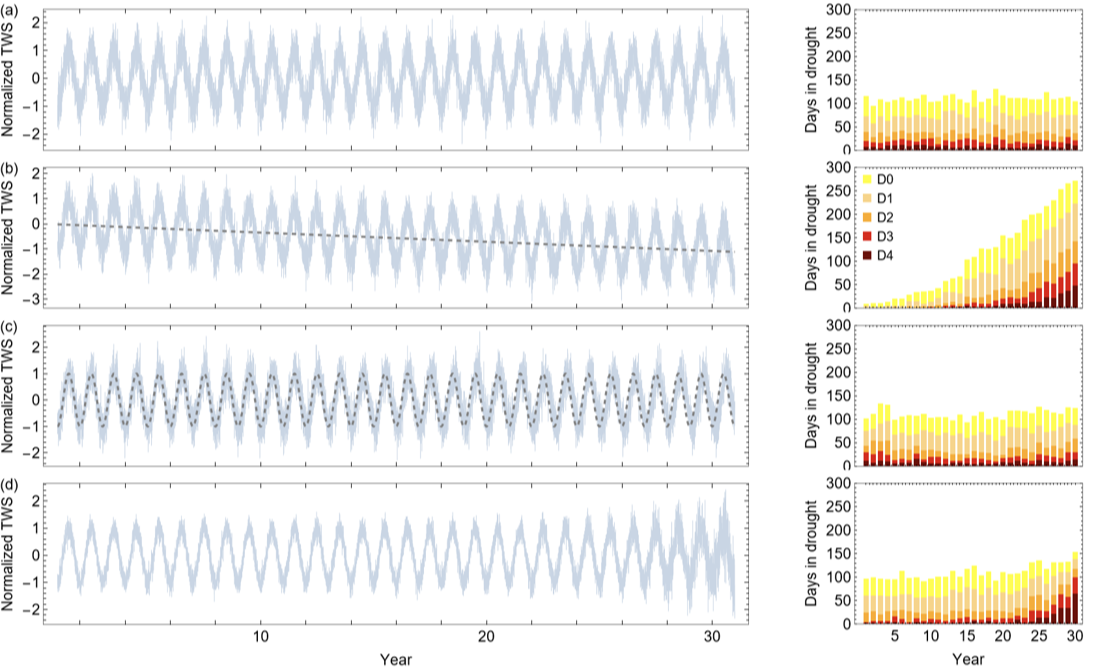
Figure 1: Before building a solution, the paper first demonstrates the problem concretely. Figure 1 shows four synthetic 30-year daily TWS time series — one stationary (the baseline) and three with different forms of nonstationarity (a drying trend, a seasonal phase shift, and an increase in variance) — and applies the conventional percentile-based drought metric (as used in the U.S. Drought Monitor) to each. This sets the stage for the entire paper: even visually, it is clear that a metric designed for a stable world produces wildly different drought counts when the underlying system is changing. This motivates the need for a rigorous mathematical framework to quantify and understand these errors.
Generate the positions of days within 30 years that are included for the estimation of percentile based drought for each Day of Year
In[]:=
DOYn30YR=Flatten[Table[{365,365,365,366},{i,8}]][[1;;30]];DOY366Pos30YR=Join[Table[Join[{j},Table[j+Total[DOYn30YR[[1;;i]]],{i,29}]],{j,59}],{Flatten[Position[DateRange[{2001,1,1},{2030,12,31}],DateRange[{#,2,29},{#,2,29}][[1]]]&/@{2004,2008,2012,2016,2020,2024,2028}]},Table[Join[{j},Table[j+Total[DOYn30YR[[2;;i]]],{i,2,30}]],{j,60,365}]];DOYclimPos30YR=Join[{Union[Sort[Join[DOY366Pos30YR[[1]],DOY366Pos30YR[[2]],DOY366Pos30YR[[3]],DOY366Pos30YR[[-1]],DOY366Pos30YR[[-2]]]]]},{Union[Sort[Join[DOY366Pos30YR[[2]],DOY366Pos30YR[[3]],DOY366Pos30YR[[4]],DOY366Pos30YR[[1]],DOY366Pos30YR[[-1]]]]]},Table[Union[Sort[Join[DOY366Pos30YR[[i]],DOY366Pos30YR[[Mod[i+1,366,1]]],DOY366Pos30YR[[Mod[i+2,366,1]]],DOY366Pos30YR[[i-1]],DOY366Pos30YR[[i-2]]]]],{i,3,366}]];DOYclimPos30YRfinal=Join[DOYclimPos30YR[[1;;57]],Table[Sort[Join[DOYclimPos30YR[[da]],Flatten[Table[Position[DateRange[{2001,1,1},{2030,12,31}],DateRange[#,#][[1]]]&/@{{i,3,da-57}},{i,{2001,2002,2003,2005,2006,2007,2009,2010,2011,2013,2014,2015,2017,2018,2019,2021,2022,2023,2025,2026,2027,2029,2030}}]]]],{da,58,62}],DOYclimPos30YR[[63;;366]]];
Create a function to calculate percentile based drought
In[]:=
DOYn=Flatten[Table[{365,365,365,366},{i,8}]][[1;;30]];DOYIND=Flatten[Table[Range[1,DOYn[[i]]],{i,30}]];GetDroughtPercentile[input_(*timeserieswithoutdates*),inputDateRange_]:=Module[{inputdateTS,DOYpercentilePOOL,TSconvertedPercentile},inputdateTS=Transpose[{inputDateRange,input}];DOYpercentilePOOL=Table[Quantile[input[[DOYclimPos30YRfinal[[i]]]],#/100]&/@Range[100],{i,1,366}];TSconvertedPercentile=Flatten[Table[Position[DOYpercentilePOOL[[DOYIND[[i]]]],Nearest[DOYpercentilePOOL[[DOYIND[[i]]]],input[[i]]][[1]]],{i,Length[DOYIND]}]];TSconvertedPercentile];
Define the relative percentile ranges for five different drought levels
In[]:=
DroughtLevel={{20,30},{10,20},{5,10},{2,5},{0,2}};(*ConstructtimeseriesshowninFig.1.*)TSexample1=Table[Sin[2*Pi/365.25*t-0.5*Pi],{t,Length[DateRange[{2001,1,1},{2030,12,31}]]}]+RandomVariate[NormalDistribution[0,0.4],Length[DateRange[{2001,1,1},{2030,12,31}]]];TSexample2=Table[Sin[2*Pi/365.25*t-0.5*Pi]-0.0001*t,{t,Length[DateRange[{2001,1,1},{2030,12,31}]]}]+RandomVariate[NormalDistribution[0,0.4],Length[DateRange[{2001,1,1},{2030,12,31}]]];TSexample2b=Table[Sin[2*Pi/365.25*90-0.5*Pi]-0.0001*t,{t,Length[DateRange[{2001,1,1},{2030,12,31}]]}];TSexample3=Flatten[Table[Sin[2*Pi/365.25*t-Pi/2-2*Pi/365.25*1.7*yr],{yr,30},{t,1,DOYn[[yr]]}]]+RandomVariate[NormalDistribution[0,0.4],Length[DateRange[{2001,1,1},{2030,12,31}]]];TSexample3b=Table[Sin[2*Pi/365.25*t-0.5*Pi],{t,Length[DateRange[{2001,1,1},{2030,12,31}]]}];TSexample4=Table[Sin[2*Pi/365.25*t-0.5*Pi],{t,Length[DateRange[{2001,1,1},{2030,12,31}]]}]+Flatten[Table[RandomVariate[NormalDistribution[0,Exp[yr/3]/50011.1+0.212],DOYn[[yr]]],{yr,1,30}]];(*Estimatingdaysindroughtperyearfortheconstructedtimeseries*)DPTSexampleall(*droughtpercentiles*)=GetDroughtPercentile[#,DateRange[{2001,1,1},{2030,12,31}]]&/@{TSexample1,TSexample2,TSexample3,TSexample4};DITSexampleall(*droughtlevels*)=Table[Cases[Transpose[{DateRange[{1,1,1},{30,12,31}],#}],{{__},_?(DroughtLevel[[i,1]]<#≤DroughtLevel[[i,2]]&)}],{i,5}]&/@DPTSexampleall;DIyrcountTSexampleall(*daysindroughtperyear*)=Table[Length[Cases[#[[level]],{{yr,__},_}]],{yr,30},{level,5}]&/@DITSexampleall;
Plot out Fig .1 .
Figure1=TableFormGridPartitionMapThreadOverlay[{##}]&,{#,Style["("~~#~~")",FontFamily"Helvetica",FontSize14]&/@CharacterRange["a","z"]〚1;;Length[#]〛}&@MapThreadDateListPlot#1,{1,1,1},&,{{TSexample1,{TSexample2,TSexample2b},{TSexample3,TSexample3b},TSexample4},{3.5,3.5,3.5,40}},UpTo[1],ItemSizeFull,TableFormMapThreadBarChartReverse[#1,2],&,{DIyrcountTSexampleall,{3.5,3.5,3.5,40},{"",Placed[{"D4","D3","D2","D1","D0"},{Left,Top}],"",""}}
Out[]//TableForm=
Part 2: Bias-variance decomposition framework
Part 2: Bias-variance decomposition framework
Figure 2: With the problem established, Figure 2 introduces the paper’s core analytical tool: bias-variance decomposition. Focusing on a single illustrative case — estimating an exceptional (D4) drought on April 1 of year 30 — the figure walks through how bias (systematic error) and variance (uncertainty) each respond to the choice of climatology length and sample density, across all four scenarios from Figure 1. The key insight is that these two error sources trade off against each other: using more data reduces variance but can increase bias when the system is nonstationary. The orange shading highlights the “sweet spot” — the optimal climatology length that minimizes total error — which shifts substantially depending on the type and severity of nonstationarity. This figure is the theoretical heart of the paper.
Create function to calculate total errors and errors from bias and variances as a function of
1) climatology length
and
2) sample density and plot them out
1) climatology length
and
2) sample density and plot them out
ClimLengthSquareLossBiasVarianceEstimationPLOTwSampleDensity[inputPART_(*deterministicpartofthesampledata*),QuantileSelection_(*levelofdrought*),climYRLengthRange_(*lengthofclimatology*),SampleRadius_,simulationSize_,YRnoiseSTD_(*noisepartofthesampledataperyear*),DOYinterest_,ParamLabel_,Legend_,GridLineFlag_,PlotTSR_,PlotR_(*plotrangeminandmax*)]:=Module{QtrueDATEx,DOYcorepos,DOYsamplepos,INPUTsample,Phat,biasDATEx,varDATEx,squarelossDATEx,optimalCLIMLENGTH,MinsquarelossDATEx},QtrueDATEx=Quantile[NormalDistribution[inputPART[[DOYclimPos30YRfinal[[DOYinterest]]]][[-3]],YRnoiseSTD[[-1]]],QuantileSelection];DOYcorepos=DOYclimPos30YRfinal[[DOYinterest]][[3;;-1;;5]];DOYsamplepos=Sort[Flatten[Join[Table[DOYcorepos+i,{i,SampleRadius}],{DOYcorepos},Table[DOYcorepos-i,{i,SampleRadius}]]]];INPUTsample=Table[inputPART[[DOYsamplepos]]+Flatten[Table[RandomVariate[NormalDistribution[0,YRnoiseSTD[[i]]],(SampleRadius*2+1)],{i,30}]],{ir,simulationSize}];Phat(*relativefrequncyofhsampleswithvalues<Qtrue*)=Table[(Count[#[[-Lyr*(SampleRadius*2+1);;-1]],n_/;n≤QtrueDATEx]/((SampleRadius*2+1)*Lyr))&/@INPUTsample,{Lyr,climYRLengthRange[[1]],climYRLengthRange[[2]]}];biasDATEx=(Mean[#]-QuantileSelection)^2&/@Phat;varDATEx=Variance[#]&/@Phat;squarelossDATEx=Mean[(#-QuantileSelection)^2]&/@Phat;MinsquarelossDATEx=Min[squarelossDATEx];optimalCLIMLENGTH=Range[climYRLengthRange[[1]],climYRLengthRange[[2]]][[Position[squarelossDATEx,Min[squarelossDATEx]][[1,1]]]];ShowDateListPlotTranspose[{DateRange[{1,1,1},{30,12,31}][[DOYsamplepos]],#}]&/@Transpose[Table[Quantile[INPUTsample[[All,i]],{0.25,0.5,0.75}],{i,Length[DOYsamplepos]}]],,DateListPlotCases[Transpose[{DateRange[{1,1,1},{30,12,31}][[DOYsamplepos]],#}],{{_?((30-Range[climYRLengthRange〚1〛,climYRLengthRange〚2〛]〚Position[squarelossDATEx,Min[squarelossDATEx]]〚1,1〛〛)<#≤30&),__},_}]&/@Transpose[Table[Quantile[INPUTsample[[All,i]],{0.25,0.5,0.75}],{i,Length[DOYsamplepos]}]],,ListPlot(Transpose[{Range[climYRLengthRange〚1〛,climYRLengthRange〚2〛],#1}]&)/@{biasDATEx,varDATEx,squarelossDATEx},
Construct time series separately for the deterministic part and noise part
In[]:=
DOYinterest=92;TSexample1PART=Table[Sin[2*Pi/365.25*t-0.5*Pi],{t,Length[DateRange[{2001,1,1},{2030,12,31}]]}];TSexample1Noise=Table[0.4,{yr,30}];
Nonstationary Case with Trend
In[]:=
TSexample2PART=Table[Sin[2*Pi/365.25*t-0.5*Pi]-0.0001*t,{t,Length[DateRange[{2001,1,1},{2030,12,31}]]}];TSexample2Noise=Table[0.4,{yr,30}];
Nonstationary Case with seasonal shift
In[]:=
DOYn=Flatten[Table[{365,365,365,366},{i,8}]][[1;;30]];TSexample3PART=Flatten[Table[Sin[2*Pi/365.25*t-Pi/2-2*Pi/365.25*1.7*yr],{yr,30},{t,1,DOYn[[yr]]}]];TSexample3Noise=Table[0.4,{yr,30}];
Nonstationary Case with shift in variance
In[]:=
TSexample4PART=Table[Sin[2*Pi/365.25*t-0.5*Pi],{t,Length[DateRange[{2001,1,1},{2030,12,31}]]}];TSexample4Noise=Table[Exp[yr/3]/50011.1+0.212,{yr,30}];
Plot out Fig .2 .
Part 3: Errors in drought assessment in response to nonstationarity
Part 3: Errors in drought assessment in response to nonstationarity
Figure 3: Figure 2 examined specific illustrative cases; Figure 3 zooms out to explore how drought estimation errors behave systematically across the full parameter space of nonstationarity observed globally. Three panels cover the three types of nonstationarity (trend, seasonal shift, variance change), each showing how total error evolves with climatology length for both all droughts (D0–D4) and exceptional droughts (D4) under two sampling densities. A critical asymmetry emerges: for moderate droughts, error spread grows as nonstationarity intensifies (high uncertainty, different reference periods give very different answers); for D4 droughts, error spread actually collapses as drying trends intensify — the bias is so dominant and consistent that all reference period choices converge on the same wrong answer. This figure provides the theoretical backbone for interpreting the global results that follow.
Create function to estimate errors in bias - variance decomposition for sample density of 5 - days
Create function to estimate errors in bias-variance decomposition for sample density of 31-days
Generate simulations with 5-day sample density, 10000 realizations for each case
Generate simulations with 31-day sample density, 10000 realizations for each case
Plot out Fig .3 .
Part 4: Impact of nonstationarity in drought assessment: Application to global reanalysis TWS
Part 4: Impact of nonstationarity in drought assessment: Application to global reanalysis TWS
Figure 4: Figure 4 quantifies the actual drought assessment errors across the globe for the exceptional drought category (D4) — the most consequential for disaster declarations and emergency responses. Panel A shows the median bias: across much of the Middle East, Central and South Asia, and parts of Australia, assuming stationarity leads to D4 drought days being estimated at 10–50+ times their expected value (massive overestimation). Panel B shows the relative uncertainty (IQR): strikingly, the regions of highest uncertainty do not simply mirror the regions of highest bias. Western North America, southeastern Brazil, and parts of High Mountain Asia show the greatest sensitivity to reference period choice despite moderate bias — meaning drought assessments there are not necessarily wrong on average, but are highly unstable depending on which years of data are used as the baseline.
Read in the land mask file, greenland and glacier mask file, and the median and IQR of number of days in file for the last year
Calculate the median BIAS and relative IQR
Plot out Fig .4 .
Figure 5: This analysis synthesizes the global results into a single diagnostic relationship, plotting median bias against relative uncertainty (IQR) for all drought levels (D0–D4) across every grid cell on Earth. This reveals a characteristic nonlinear signature: uncertainty is highest when bias is near zero (i.e., when the system is marginally nonstationary, making reference period choice most consequential), and diminishes when bias is very large (i.e., when the trend is so strong that all reference periods agree on the wrong answer). This relationship is more pronounced for lower drought levels (D0–D1) than higher ones, and peaks for D4 at around 26 times the expected drought days before collapsing. This figure powerfully encapsulates the paper’s central message: nonstationarity does not simply shift drought estimates in one direction — it introduces a complex, level-dependent interplay between systematic error and uncertainty that conventional methods are less prepared to handle.
Partition the median BIAS into uneven bins
Plot out Fig .5 .
CITE THIS NOTEBOOK
CITE THIS NOTEBOOK
Anthropogenic influences on the water cycle amplify uncertainty in drought assessments
by Wanshu Nie, Sujay Kumar & Long Zhao
Wolfram Community, STAFF PICKS, April 21, 2026
https://community.wolfram.com/groups/-/m/t/3699762
by Wanshu Nie, Sujay Kumar & Long Zhao
Wolfram Community, STAFF PICKS, April 21, 2026
https://community.wolfram.com/groups/-/m/t/3699762