Control of a Constant-Volume Blender
Authors: Housam Binous and Ahmed Bellagi
Control of a Constant-Volume Blender
Authors: Housam Binous and Ahmed Bellagi
Authors: Housam Binous and Ahmed Bellagi
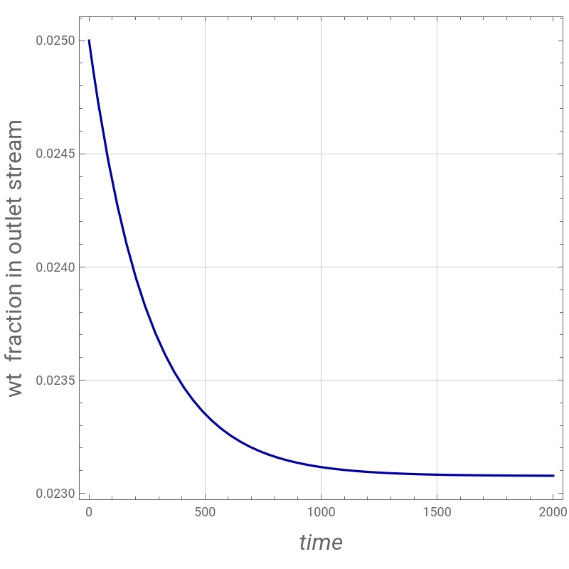
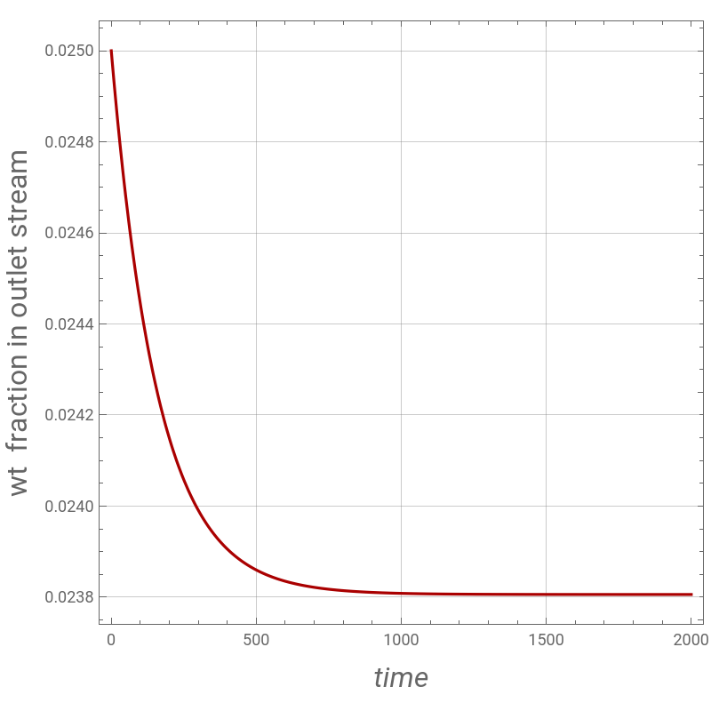
Figure below shows a sketch of a blender.Total material balance is :Partial material balance is :where x is the weight fraction of component A. We assume the system is dilute. Hence, ρ ≈ constant.The problem is a MIMO. However, if we assume =0 (i.e. V is constant by using an overflow line) then and we recover a SISO problem.Here, we propose to control the weight fraction of component A in the blender outlet stream, , by manipulating the mass flow rate of stream 2 (labeled w2).. Note that we apply a negative gain to invert the controller response. Indeed, when e(t) is positive, the controller has todecrease w2.Given: V=A h=1 m3, x1=0.1, x2=0, w1=1, w2=3, w2n=3, ρ=1000. We suppose that the mass flow rate of stream 1, w1, is decreased to 0.9 at t=0.For each one of the scenarios below, we plot the weight fraction of A in the outlet stream and flow rate versus time.1. there is no control action.2. A P-controller is used to control the weight fraction of A in the outlet stream. Controller gain is Kc = 100. =0.025wt %.3. A PI-controller is used to control the weight fraction of A in the outlet stream. Controller gain is Kc = 10 and the reset time is τI = 2. 4. If w1 is kept equal to 1 at all times and the set point is fixed equal to 0.045 at t=0. A PI-controller is used to control the composition of the outlet stream. Controller gain is Kc = 10 and the reset time is τI = 5.Acknowledgement:Largely inspired from LearnChemE, Process Controls screencasts, Prof. Martha Grover : https://learncheme.com/screencasts/process-controls/
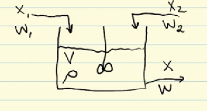
ρA=ρ==w1+w2-w
h
t
V
t
m
t
ρV=w1x1+w2x2-wx
x
t
V
t
w=w1+w2
x
w2=w2n-e(t)+e(t)twithe(t)=-x(t)
K
c
1
τ
I
x
sp
w
sp
Open loop response or no control action
In[]:=
ss=Flatten@NSolve[{w1x1+w2x2wx,ww1+w2},{x,w}]
Out[]=
x,ww1+w2
w1x1+w2x2
w1+w2
In[]:=
x1=0.1;x2=0;
In[]:=
w1=1;w2=3;
In[]:=
ss
Out[]=
{x0.025,w4}
In[]:=
rho=1000;V=1;
In[]:=
w1=If[t<0,1,1×0.9]
Out[]=
If[t<0,1,1×0.9]
In[]:=
sol=NDSolve[{rhoVx'[t]w1x1+w2x2-(w1+w2)x[t],x[0]0.025},x,{t,0,5000}]
Out[]=
xInterpolatingFunction


In[]:=
Plot[x[t]/.sol,{t,0,2000},PlotRangeAll,PlotStyleDarker@Blue,FrameTrue,GridLinesAutomatic,AspectRatio1,ImageSize400{1,1},FrameLabel{Style["time",16,Italic],Style["wt fraction in outlet stream",16]}]
Out[]=
In[]:=
x[t]/.sol/.t5000
Out[]=
{0.0230769}
In[]:=
0.90.1/3.9(*check*)
Out[]=
0.0230769
Closed loop response - proportional only control action
In[]:=
w2ss=3;
In[]:=
Kc=100;
In[]:=
w2=w2ss-Kc(0.025-x[t])
Out[]=
3-100(0.025-x[t])
In[]:=
sol=NDSolve[{rhoVx'[t]w1x1+w2x2-(w1+w2)x[t],x[0]0.025},x,{t,0,5000}]
Out[]=
xInterpolatingFunction

In[]:=
Plot[x[t]/.sol,{t,0,2000},PlotRangeAll,PlotStyleDarker@Red,FrameTrue,GridLinesAutomatic,AspectRatio1,ImageSize400{1,1},FrameLabel{Style["time",16,Italic],Style["wt fraction in outlet stream",16]}]
Out[]=
Closed loop response - proportional-integral control action
Closed loop response - proportional-integral control action - response to a set point change